From Lines To Angles, and Particles To Rigid Bodies

We dove straight into circular motion with the 2nd year students this past week. The primary focus of last year was linear dynamics and although we did study objects that moved along curved paths (projectiles), we were still looking at two-dimensional motion as being composed of two component motions along straight lines.

In the second year program, a good part of the first semester is dedicated to looking at objects that rotate around a central axis. There are two major shifts that will be introduced. The first is the introduction of an entirely new coordinate system – polar coordinates. The students spent most of last year learning about two dimensional vectors in Euclidean space, but this year, we will see that for objects traveling in various curved paths, a polar coordinate space can actually be much easier work with. The other shift will introduce students to collections of particles composed into continuous rigid bodies. This requires some significant changes in how the students view an object’s orientation in space and how an object’s mass is distributed. No longer can we assume that the object’s mass is located at a single point in space. In both cases, we are adding to the complexity of our conception of the universe by adding new representations of both space and the objects that inhabit that space.

Observing Circular Motion

In the modeling pedagogy, a new concept or collection of concepts is introduced using a paradigm lab. These labs are meant to introduce students to a new phenomenon and to be the launching off point of the actual building of a conceptual model.

Using the video analysis and vector visualization tools of LoggerPro, I had the students track the motion of a Styrofoam “puck” that was placed on our air hockey table (yes, we actually have an air hockey table that was donated to the school!) but was also attached to a thin thread to a fixed point on the table. The students used the video to track the motion of the puck as it essentially traveled in a circular path.

Although the lab is a bit tricky to set up, the ability to not only track the position of the object in two dimensions, but also the ability to attach velocity and acceleration vectors to the object is really helpful in engaging students in a great conversation around why the acceleration vector points to the inside of the circle. It also allows us to discover a whole new set of mathematical functions for describing motion. After tracking the position of the puck, we are ready for a class white board discussion.

The Graph Matching Mistake Game

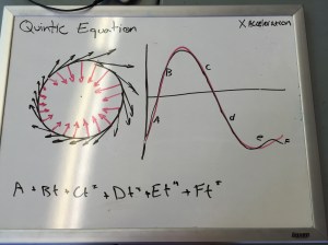
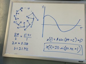
I ask the students to draw the motion map of the puck’s motion in two dimensions including the velocity and acceleration vectors. I then ask them to include the graphs created by LoggerPro. LoggerPro produces a really interesting position vs. time graph in both the x and y dimensions. At this point the class knows the drill, and they use the mathematical function matching tool in LoggerPro to match the graph. I ask the students to include on their whiteboards the function that they think best fits the plotted data. This is where it gets really interesting.

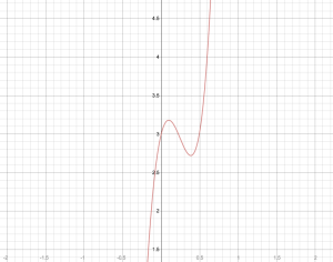
Notice in the above photo that the students used a polynomial function. I then ask the students to use Desmos to plot their graphs. Then I ask them to zoom out on the graph.

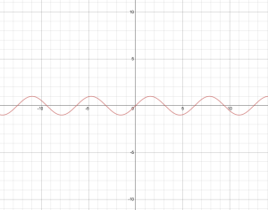
This is where they discover how this function can’t explain the position vs time data for an object that continually repeats the same path. Some of the students in the class recognize that the data is better explained using a sine function. Because not all the students have been introduced to this function, it presents an opportunity for some students to teach the other students about how these functions work.

I allow the students to explore the sine function in Desmos, asking them to change the coefficients of the function in order to discover how these coefficients affect the graph.

The next step is to investigate more thoroughly the relationship between the acceleration and the velocity, as well as introduce the benefits of using polar coordinates to describe how an object’s position changes when you are dealing with an object that is traveling in a circular path. Desmos has the ability to change the graph type from the x,y coordinate plate to a polar representation. We discuss the difficulty of representing an object’s circular path using x(t) and y(t) functions as opposed to r(t) and theta(t) because r(t) is just a constant.

Next up, trying to answer the question: “If it’s accelerating inward, then why isn’t it speeding up towards the inside of the circle?!” Once again, the difficult concept of inertia…