Computational Deployment: Simulating A Rocket

The model rocket project has long been a favorite at the Academy. For the past fifteen years, students have designed, fabricated and then launched model rockets as the first project of the program. Over the years, I have tweaked the project several times, each time finding new ways to introduce authentic analysis in the process.

This year I have taken a deep dive into computational modeling, and as part of the rocket project, students were asked to create a simulation of their rocket prior to launch. In this post I will discuss how I did this, and how it turned out.

Simulating The Momentum Principle:

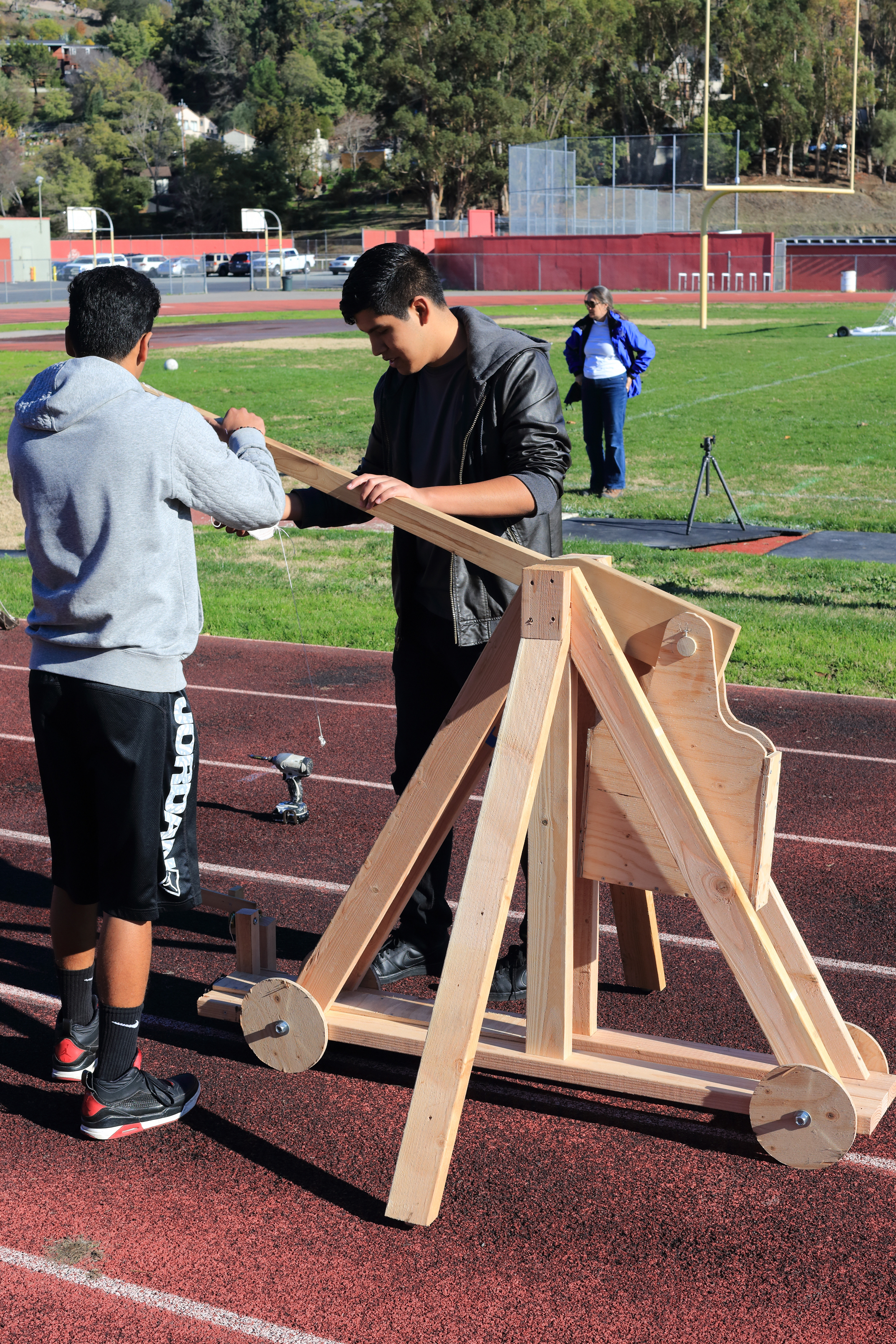
Prior to getting started on this, students investigated the causal relationship between forces and changes in motion. Using force sensors, carts, weights and elastic cords of different lengths, students began building a qualitative and quantitative model relating the momentum of a particle to the forces acting on the particle.

Screen Shot 2018-12-22 at 9.27.05 AM

In previous years, I waited to introduce momentum until after a significant amount of time was spent on forces, balanced and unbalanced. This year I decided to go directly to momentum. This is a bit of a break from the established modeling instruction sequence, but I think its a good alternative that is also suggested by the great textbook Matter and Interactions. The momentum principle can easily be modeled computationally and I think the students are able to grasp it conceptually.

I have included a link to a Google Doc that is the introductory activity that I created. My approach here, as it has been with this entire unit is to give the students guided questions that allow the students to discover and investigate the code required to simulate the momentum principle. This is my first attempt, and I am sure it will undergo many revisions:

Simulating The Momentum Principle

Introducing Conditional Behavior

One of the really great things about building a simulation of a rocket has three distinct phases of its trajectory – the thrust phase, the cruise phase and the descent phase. This gives the students three different phenomena to study and simulate: positive acceleration when two unbalanced forces are acting on the rocket during the thrust phase, free fall when the fuel runs out, and then constant velocity when the parachute has been deployed.

In order to simulate this, students needed a way to change the forces acting on the rocket at different time intervals. This is done using a conditional statement:

If This Then That

Conditional statements are very easy to create in Tychos – but they work a bit differently from other programming interfaces. Here is an example:

# The thrust force - F (thrust, rocket, fuel)
Ftrf = if (t < 1.8, [0, 6], [0, 0])

In this code snippet, a force is given a different value based on a condition, in this case whether the time in the simulation is less than 1.8 seconds. If it is, then the force is given a positive 6 value in the Y direction, and if the time is greater than 1.8 seconds, then the force becomes zero.

This allows the students to simulate the thrust phase of the rocket by having the thrust force disappear once the fuel has run out. We conducted tests on Estes C6-5 rocket engines in order to establish the time value. You can read more about how we did this here.

The students did the same thing to figure out when the parachute should deploy. Again this was established based on information from Estes as well as our own tests.

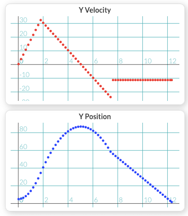
Comparing Simulation Data to Real Data

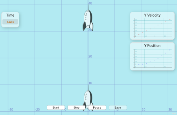
The students could analyze the simulated rocket behavior by using the graphing tools in Tychos. The students graphed the vertical velocity as well as the vertical position of their simulated rockets. Here is an example of what those graphs look like:

Screen Shot 2018-12-22 at 10.22.21 AM

The last step of the process was for the students to compare their simulated data to the real data that was captured by the altimeter that we use in the rocket’s payload. Below are two images of the graphs of the data they retrieved from the rocket’s altimeter:

rocket_v_graph

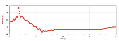
velocity data from altimeter – imported into LoggerPro

rocket_y_graph

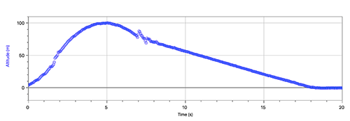
altitude data from altimeter – imported into LoggerPro

The shapes of the graphs from the simulated data and the real data are very similar! That was certainly exciting to see that the simulations were at least giving results that qualitatively matched the real behavior of the rockets.

Two factors that certainly created significant discrepancies between the real rockets and the simulated rockets was the existence of air resistance on the real rocket, and the fact that the real rockets didn’t always go perfectly straight up! We plan on modifying the simulations, but that will have to wait for a future post.

The Great (Mini) Robot Race

Robotics – The Synthesis Project

The final project of the two year academy program requires that the students design, fabricate, program and test an autonomous robot. We have been doing this project since the inception of the program, but this year we have made some significant improvements on the project. In this post I will explain the project, and highlight those improvements.

This project is an extremely challenging task that requires successfully completing several “sub-projects”. We tell the students at the beginning of the school year, that this project is more difficult than any of the other projects – by a long shot!

“If you haven’t done everything, then you haven’t done a thing.” – Red Whittaker

We completely changed our robot competition parameters this year. In previous years we had the students design sumo wrestling battle bots. Although this was a fun project, we started to notice that some robots performed really well without really having to “think”. These robots generally lumbered around the ring, sometimes without even actually “seeing” their opponents. Through pure luck they just managed to push their lighter opponents out of the ring. We decided that we needed to change the project in order to force teams to be smarter and we also wanted to get away from a robot competition that seemed to focus on aggressive battle.

Ironically, I suppose, our robot project changes were inspired by the classic Nova film that documented the DARPA challenge known as the Great Robot Race. In this race, the autonomous vehicles raced through the Mohave dessert on a course that was revealed to the competitors only hours before the beginning of the race.

Bob set about building an impressive “maze” for the robots to navigate. The robots had to make their way through a series of 90 degree turns defined by a series of connecting corridors with vertical walls about 20 cm tall. The robots were then given two attempts to make it through the course as fast as they could.

The Brains and Braun

When we first started this project about twelve years ago, we first used a Java based board that we liked, but it was really expensive and we didn’t really need much of the hardware and software features that it offered. About eight years ago, the Arduino board was taking the Maker community by storm and we decided to hop on the Arduino bandwagon, and we have been very happy ever since. The simplicity, online community, the plethora of code examples and tutorials as well as the price have been key points in why we have decided to keep using the Arduino. This year we decided to incorporate DC motors from Sparkfun and Adafruit’s motor shield. The combination allowed the students more flexibility regarding drive train design, and also allowed for some interesting discussions around the advantages and disadvantages of servos vs dc motors. Our only complaint with the shield would be that it would be nice to have the headers pre soldered!

Designing The Circuitry

fritzing-preview-pcb

One of the major additions to the project was to require that students design and fabricate the circuitry for their robots. We did this by introducing two new skills to the project. Students had to learn how to use a printed circuit board (PCB) design software known as Fritzing, and then they had to learn how to fabricate their PCB boards using a CNC mill.

There are a number of amazing PCB design tools out there – and many are free! They all have their strengths and weaknesses. Here is what we found out as we did our research to find the right tool.

Autodesk’s Circuits is great because its web based, super easy to use and has an amazing feature where you can actually simulate the circuit. You can add a virtual voltmeter of ammeter to your virtual circuit and then with a push of a button, you can get virtual readings on the meters. I found this tool to be amazing for teaching circuitry and I allowed the students to use it as a “key” for their worksheets. It also has the ability to simulate an Arduino too! You can add an Arduino to your project, connect up LED’s, servos, etc. and actually see them light up or rotate as you change the code. It is a bit limited in that it doesn’t support most added libraries, but it is still amazing. We eventually decided not to use it for PCB design because it is unfortunately a bit clunky and doesn’t allow for much customization of the board.

Eagle is of course one of the most advanced and feature rich PCB design tools out there. It is also very complicated. IT of course offers the largest toolset, complete control of the design process and the free version is as close to a professional tool as one could hope for. The problem is that all these features come at a price – complexity. If we had an entire year to spend on this project, I might have decided to go with this tool, but we needed something that the students could learn quickly and weren’t going to get frustrated with…

Fritzing is a free, open source “beta” software that is very similar in look and feel to Autodesk’s Circuits – in fact I think Autodesk’s product must have been inspired by Fritzing? Although Fritzing lacks the amazing simulation tools that Autodesk Circuits has, it does offer a much better PCB design environment. The options that are available for editing the component foot prints, the PCB attributes, etc. make it really nice to work without making the tool too complex. This is the tool we decided to teach and use in class, and the students liked it.

pcb-milling-opener

Fabricating The Circuitry

Back in the fall we decided to invest in a small CNC mill produced by a local company out of San Francisco named Other Machine Co. This machine, called the OtherMill has been an amazing addition to the lab. With this machine, we have been able to teach the students how to fabricate their own PCB’s. The OtherMill is not just for PCB fabrication, in fact we have used it to mill small aluminum parts as well.

2323-00

This micro CNC desktop mill is super easy to setup, really easy to use and plays really nicely with Fusion 360 – our 3D CAD and CAM software. I was incredibly surprised and pleased by how easy it is to learn the operating software – known as OtherPlan. The company has a great support website full of great tutorials, and we were able to teach all the students how to use the machine in just a few days.

The PCB files generated by Fritzing (we exported them as Gerber files) worked flawlessly with the OtherMill, and within a very short period of time, all the students had designed and fabricated single sided PCB boards for their robots.

img_3283

The Final Results

As with any major changes to a project, there are lessons to be learned. We realized that the task was rather complicated and many of the students did not make it as far through the course as they had hoped. It was clear however that this competition proved more interesting from the perspective of getting students to see the importance of software design. Not only did we see very different software strategies, but the variance in hardware design was surprising. They really had to think about how the hardware and software had to work together, and they had to think about optimization. This was a clear advantage of this competition over the previous year’s competitions. Students spent far more time trying to figure out how they were going to shave time off their attempts, and how they were going to adjust software and hardware to better navigate the course. From our perspective, the changes to the project proved to be fantastic, and we are looking forward to improving on the project design for this year. Some of the things that we are going to do this year is introduce some different sensors for the students (like “feelers”) and also give them a price list and budget so that they have more hardware choices.

Our Custom Designed Bridge Tester

Our Goal – Make A Better Bridge Crusher!

This year Bob and I decided to upgrade our bridge project. We wanted to create an improved device for measuring the load on the model bridges created by the students. Specifically, we wanted to design a way for the students to collect meaningful performance data.

The problem with our old method (filling a bucket with sand until the bridge catastrophically failed) was that it didn’t allow for the students to collect evidence about where and why the bridge failed. In many cases, the bridge actually experienced a significant failure, but because the bridge collapsed around the loading plate, the loading plate actually acted as a support for the bridge.

We had seen other “bridge testers” from vendors (http://www.pitsco.com/Structures_Testing_Instrumenthttp://kelvin.com/kelvin-bridge-material-tester-w-cpad/http://www.vernier.com/products/sensors/vsmt/) but we had the idea that perhaps we could create one that might be better, or at least it might be fun to try. In this post, we are going to share with you what we created and why we think it actually turned out really well, but we also point out some room for improvement.

The Frame

The frame of the entire device is really based on the Vernier Structures and Materials Tester. We thought this frame was probably the best, and we wanted to make our tester from extruded aluminum tubing as well. We went about designing the bridge tester in our favorite CAD program, Fusion360 by Autodesk. We sent our CAD file to the company 8020 and they precut all our t-slotted aluminum frame members to size. This was awesome because it made assembly super easy and it saved us on shipping too! Our experience with this company was amazing – they were super helpful and even gave us some really helpful advice. If you are thinking about making anything requiring t-slotted aluminum, definitely order from them.

The Load Sensors

We wanted a a bridge tester that actually gave us data that allowed us to figure out how and why the student bridges failed. That meant that we needed more data and we needed data that could be connected to the design and fabrication of the bridge. We noticed that all the vendors’ designs had only one load sensor, and some also had a way to detect overall deflection. We suspected that we could get better data if we had four independent load sensors – one for each abutment where the bridges were supported. The four sensors would (theoretically) give the students a way to analyze how the load was being distributed, and thus tell us something about the torsional behavior of the bridge.

Sparkfun load sensor

Sparkfun load sensor

I set out to learn a bit about load sensors and I came across a fantastic tutorial at Sparkfun (https://learn.sparkfun.com/tutorials/getting-started-with-load-cells). We ordered four load sensors (see picture above) from Sparkfun. Our design (shown below) has the four load sensors  fitted with 3D printed “shoes” as the bridge abutments.

IMG_3048

The four load cells.

IMG_3044

Two load cells with abutments.

The sensors are mounted on custom fabricated aluminum plates that can be moved laterally to accommodate slightly different bridge widths. The load sensors had to be connected to load amplifiers that were then connected to an Arduino (more on that below). The load sensors were mounted to the frame of the bridge tester on custom laser cut plates:

IMG_3043

Load cell amplifiers for two load cells.

The load amplifiers have to be used with the load sensors in order to amplify the signal so that the Arduino can read the data correctly.

The Loading Mechanism

Bob designed and fabricated the loading mechanism that was based on many of the designs we had seen online. It consists of a block that is free to move vertically up or down a threaded rod which is then connected to a spoked wheel.

IMG_3047

Loading wheel.

When the wheel is turned, the block moves up or down the threaded rod. This bar is connected to a loading plate via a metal cable that hooks into the loading plate and the block:

IMG_3053

Load plate from below – revealing loading wire attachment.

IMG_3052

Loading wire attached to threaded block.

The loading plate is placed on the loading plane of the bridge (the “roadway”), and then the bridge is loaded by spinning the wheel, which lowers the block, which pulls the bridge downwards:

IMG_3050

Loading plate on bridge.

Collecting The Data: The Software

 The software responsible for collecting the data is made up of two programs – one that runs on the Arduino micro-controller that is connected to the load sensors, and the other is a Processing sketch that runs on a computer/laptop connected to the Arduino via USB. The code is pretty simple, and it was mostly written using code from other sources and then modified for our specific purposes.

The Arduino code just collects the data from the four load sensors and then sends the data serially as a comma delimited package. The Processing code reads the serial port and then essentially dumps the data into a csv file. It does have some flourishes like a graphical display of the individual sensor loads as well as a display of the total load and whether or not the bridge has met the minimum load requirement set in the project descriptor.

You can view and download all the code here on GitHub.

The Performance Report

When the data is displayed in a graphing program, it looks like this:

Sample bridge data

Sample bridge data

You can see that the four sensors do not read equal values, and that the bridge begins distributing the load unevenly. The blue and orange lines show that these two load sensors were equally loading and were taking on a larger load than the green and red values from the other two load sensors. Later inspection of the bridge showed that this bridge failed at the load sensors that were recording a higher load value. Also, these sensors were located diagonally from one another, and once again showed that the bridge was being twisted.

You can also see that around 80 seconds (the 800 data sample) that the bridge experienced a sudden decrease in load – this was the point of failure. The data clearly shows a point at which the bridge failed and thus gives us a clear metric for performance.

The student teams were each given the results and were asked to answer these questions:

  1. What was the maximum load that your bridge sustained before failure?
  2. Calculate the load to weight ratio of your bridge.
  3. What were the individual maximum force values on each load sensor before failure?
  4. Identify on your bridge where the bridge failed. Take a picture of this point of failure and note its location.
  5. Based on the load data for the four sensors, describe why your bridge may have failed.
  6. What could you have done to increase the performance of your bridge?

The data really allowed for some rich analysis and the students were able to make some really informed critiques of their design and fabrication quality. We have been very happy with the results!

Future Improvements

For version 2.0 we hope to add these improvements:

  • Add the ability to measure deflection. We think that this might be done by measuring the angular displacement of the loading wheel, but we aren’t sure just yet.
  • Some way for the software to detect a failure – perhaps a way to detect a significant decrease in the load data. It would have to allow for some downward movement of the load data because there is some settling and deforming that can occur that might not be catastrophic.
  • It would be nice to clean up the code – especially the Processing code. I’d like to add some fancy GUI elements too so that it is a bit more attractive.

If you would like to build your own advanced bridge tester for your classroom, we can send you all our CAD files, software files and even answer questions. Its not easy to build, but its fun, and we spent about $350 dollars on this project as opposed to the $1000 to $1300 that the vendors are selling theirs for.

Simulate, Test, Analyze: A Framework For Rigor

trebuchet-launch---08_23970235271_o

“Have Fun Storming The Castle!”

At the end of this fall semester, the second year students in the Academy rolled and carried their medieval mechanisms of mayhem to the SRHS track and we spent the afternoon watching the devices hurl lacrosse balls across the athletic field.This project was the final performance assessment of the semester and required that students design a gravitationally powered projectile launcher. This is an age old engineering/applied physics project.

Like many engineering projects done in high school, the physics principles governing the dynamics of the project are quite complicated, and ultimately the actual “application” of the science principles is often cursory. Students don’t have the background or mathematical abilities to to do the complex calculations needed to make an optimization adjustment to their mechanical device.This leads to the disconnection between the science content and engineering practice. Students don’t have the ability to make an informed decision about design choices. This is because it is difficult, very difficult.

Over the past few years I have been very interested in addressing this problem. This post discusses a framework that I have been working on to incorporate science into engineering projects. I think this framework allows high school students to engage in difficult scientific analysis without overwhelming them.

A Framework For Rigor

I won’t claim that this is a perfect solution, but so far I think we have experienced some success in creating a tighter relationship between science and engineering.  Last December I helped conduct a workshop at the NCCPA Professional Development Conference in Petaluma, CA. The name of the workshop was “NGSS, Prediction Reports and Your Science Class” and the point of this workshop was to give the attendees a framework for incorporating the Engineering standards into the science curriculum.  My co-presenter (Vipul Gupta) and I focused on the creation of prediction reports using computer simulations as a way to address two very important standards in the NGSS framework:

Using Simulations with Informed Input

Computer simulations are very popular in the educational space. They give teachers and students a virtual space where students can interact with virtual lab equipment or virtual objects that behave similarly to physical objects in the real world. With that said, they can fail to address students misconceptions because they do not always succeed in linking a conceptual model to the physical behavior. I also believe that the best simulations are ones that output data that can be analyzed with other scientific/mathematical tools. I also think that a good simulation requires that students provide meaningful input that gives them opportunities for analyzing the relationship between the input and the output.

Simulations used in engineering projects can be extremely helpful in addressing one of the main problems in engineering education. Students often design and build mechanical devices without understanding the physical principles that govern the design. The design process becomes an exercise in trial and error, or simply is reduced to copying a design from the internet.

To do a predictive analysis of a rocket’s flight, or a bridge’s structural performance is extremely difficult and often requires advanced mathematics and physics. Simulations can give the students the ability to analyze their designs and understand how changing the design inputs affects the output. Once again, it is important to find a simulation that requires students to understand the inputs and outputs.

Virtual Trebuchet

For example, in our project, students were introduced to an online Trebuchet simulation tool. This simulation tool is great because it requires that the student learn how to measure and calculate certain inputs. The students must have a working knowledge of rotational inertia, center of mass, and other concepts before they use the simulation. This was ideal for our project because it gave students a relevance and motivation . They had learn about these concepts in order to actually use the simulation. The students could then change certain inputs and see how that would change the efficiency of the design, or the range of the projectile. The point is that they needed physics knowledge in order to use the tool. They might not have the ability to know how the simulation eventually calculated the output, but they knew that the simulation required an understanding of the inputs.

IMG_2674

Example Report

The Prediction Report

The next step is to ask the students to prepare a prediction report. This report is designed to get students to demonstrate their understanding of the inputs, display evidence of the required calculations or measurements needed to create the inputs and then analyze the simulation outputs. In the report for this project, I asked students to show a set of calculations and measurements for determining the center of mass of their throwing arm and the rotational inertia (moment of inertia). Students also had to provide similar information for the counterweight.  The students then had to run the simulation and document the outputs from the simulation.

The Test:  Data is Needed

The next step is to test the device. To make this step more rigorous and to be able to relate the scientific analytical process to the engineering process, it is crucial for the students to collect data that can be used to analyze the performance of their device/product and then reflect on how they would improve their design.

For this project, we decided to use high-speed video and Vernier’s LoggerPro video analysis software to plot the position of the projectile as it was launched from the device.

The Analysis

The analysis is actually broken into two parts. The first part requires a collection of calculations while the second part uses those calculations to make some qualitative assessments.

For example, in the above project, students had to use the collected position data from the video analysis tool to calculate the kinetic energy of the projectile and then the efficiency of the device. They had to be proficient at the analytical tool, which in itself requires physics content knowledge, providing once again an opportunity to apply scientific models in the analysis portion of this engineering project.

I have included the instructions for the analysis report here: Projectile Launcher Analysis Report.

Finally, students are given the opportunity to use the information gathered in the analysis report to reflect on their design, and more importantly use the information to inform how they would improve on a future design. I have included below the set of questions that I asked my students:

  1. Compare the efficiency calculation of the simulation to the efficiency rating that you calculated for your actual performance. Please describe why you think these values are not the same.
  2. Consider the design of your trigger. What design and fabrication decisions would you change in order to improve your trigger, AND explain WHY you would make those changes.
  3.  Consider the design of your sling. What design and fabrication decisions would you change in order to improve your sling, AND explain WHY you would make those changes.
  4. Consider the design of your release mechanism (called the nose). What design and fabrication decisions would you change in order to improve this mechanism, AND explain WHY you would make those changes.
  5. Consider the design of your arm. What design and fabrication decisions would you change in order to improve your arm, AND explain WHY you would make those changes.
  6. Consider the design of all other components and the overall design. What design and fabrication decisions would you change in order to improve your device (other than the trigger, sling and arm), AND explain WHY you would make those changes.

Conclusion

The overall design of this framework can be boiled down to this:

  • Engage students in a computer simulation that simplifies the process of modeling and analyzing a complex physical/chemical/biological process, but be sure that the simulation requires some conceptual and computational thinking.
  • When testing the performance of the design (bridge, rocket, etc.) make sure that the students are required to  collect data that can be analyzed and that once again demands that they apply their theoretical models.
  • Design an assessment that uses the analysis and gives the students an opportunity to make informed judgements of their designs for the purpose of redesign.

Building the Electrical Current Model with The Amazing $25 Programmable Power Supply

Not Just For Teaching Robotics

Thanks to the generous donations of supporters of the Physics Academy, we were able to purchase a new set of Arduino Uno micro-controllers for use in this year’s robotics competition. As I was planning out the unit on teaching DC circuits, I realized that some of our DC power supplies might need to be replaced. I got to thinking – could the Arduino replace these hulking, expensive power supplies?

product.exps._hero.001.590.332

The answer has been (with one caveat) – yes. The above power supplies are nice, no doubt about it, but they are big, costly ($199) and they are not as nearly as extensible as a micro-controller.

Arduino_Uno_-_R3

The Arduino micro-controller can act as a fixed 5V power supply, or using its PWM pins, you can vary the voltage from 0V to 5V with a resolution of about 20 mV. The other advantage about using the Arduino is that it gives you a chance to teach a little bit of programming too! In our case, it allows for a great introduction to robotics well before we are ready to start our unit on robotics.

The one disadvantage is that you can’t test any circuits that need over 5V of electrical potential difference, nor can you test things like motors or other higher current (> 40 mA) circuits. We didn’t find this to be a big problem, but if you do, you can actually purchase a shield (an attachment that fits on top of the Arduino) from Adafruit Industries that allows you to use a higher voltage, higher current power supply that is controllable through the Arduino.

Mapping Electrical Potential (Voltage)

One of the first activities that the students do, which is a great activity from the AMTA curriculum repository, is to have the students “map” the voltage between two metal bars that are partially submerged in water.

IMG_1870

Using the Arduino as the power supply, the students use a multimeter to check the voltage at specific locations on a grid that is placed under the transparent pan holding the water. These numbers are recorded into a spreadsheet. Excel has a great tool for doing a 3D map of the values.

potentialmap

What results is a really nice visualization of the potential isolines and the spacial variance of the voltage, and thus the electrical field.

Ohm’s Law – A Flow Model

We then move from voltage maps to flow model. The students investigate how voltage, current and resistance are related to one another. The students begin by investigating the current flowing into and out of a resistor, and most are surprised to find that the current in the same flowing into a resistor as it is flowing out. They expect that current should be “used up” by the resistor – causing a bulb to glow for example. When they find that this is not the case, they either think that they have done the experiment incorrectly or that perhaps the multimeter is not precise enough. This confusion comes from the idea that they are expecting current and energy to be equivalent.

IMG_1918

The hydrology analogy is introduced as a possible model for describing this phenomenon. We discuss the movement of water past a water wheel, and how the water flowing into the wheel is equal to the amount of water flowing “out” from the wheel. Students quickly realize that the wheel still turns, not because the water is “used up”, but because the water looses energy.

The final challenge for the students is to confront the oddity that is parallel circuits. This is made a bit easier by thinking about the flow model, but the confusion with parallel circuits stems from the idea that a battery is a constant current supplier – which of course it is not. The Arduino, just like a battery, will increase the amount of current flowing from its digital output pins when more pathways are added for the current to flow. This is where I would be careful to make sure however that you don’t approach the 40 mA limit. If you do, you can get some weird results in your observations as the Arduino will naturally cut off current draws around this range to protect its electronics.

Conclusion

The switch to the Arduino has been quite successful, and as stated before, it launches the students into the robotics project with a knowledge that the Arduino is simply a controllable power supply. They learn very quickly from that point on that the Arduino can also act like a voltmeter too! Using its analog input and switching the digital pins to be input pins, the Arduino can also mimic the functionality of a multimeter. If you are considering new power supplies, I would recommend looking into this as an option.