For the past year, I have been helping a small software development team, headed up by my friend Winston Wolff, in the creation of a web based physics simulation tool. In this blog post, I am going to describe:
- Why we started this effort,
- What we hope to achieve,
- How far we have currently progressed towards our goals,
- And invite you to try it out.
Simulations Can Be Helpful…
Many Physics teachers use computer simulations as a tool to help students learn physics. With a click of the mouse and a few keystrokes, students can quickly change the inputs to the simulation, producing different simulated behaviors of the system. This allows for quick exploration of the relationship between certain “physical” inputs and the governing dynamics of the system. Often, these explorations would be impossible to set up in the lab, or might take significant time and effort.
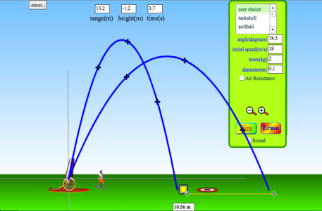
A great PHET simulation of projectile motion
…But They Have Limitations.
Although these tools can be used with a high degree of success in the classroom, the students are interacting with a virtual universe created by another human. The rules of behavior and the underlying quantitative relationships have been defined by someone else who has already done the difficult work to model the physical universe. These relationships can be inferred and they can be explored by the student, but ultimately, they are hidden behind an impenetrable wall of software code. There is also a certain faith that the student must have in the simulation – there must exist an acceptance that the simulation creators did their job correctly.
Students Coding Their Own Simulations is Awesome…
Some highly regarded physics educators have introduced the practice of teaching computer programming in the physics classroom. The advantage of engaging students directly in the construction of simulations, according to Ruth Chabay and Bruce Sherwood
“is that there are no “black boxes”: students write all of the computational statements to model the physical system and to visualize the abstract quantities.”
Additionally, they argue that having students gain some experience and exposure to computational modeling
“in the form of programming, even at the introductory level, can be an important component of a general education for living in today’s world.”
Giving students the opportunity to write their own simulations gives them the ability to engage in computational physics directly and to give them vital experience in one of the aspects of being a scientist – namely writing some code.
… But There Are Challenges For Teaching Coding.
Although there are great reasons for integrating computer science with Physics, and therefore developing students’ understanding and experience with computational Physics, there are some significant challenges for the teacher.
Teaching students to code their own physics simulations is not trivial. It requires significant instructional time, even given the fact that there are some amazing tools and frameworks for graphics programming (VPython, Processing). Chabay warns that time spent on teaching computer science principles and practices needs to be assessed against the time lost teaching and learning physics.
Due to the complexity and in many cases, the lack of exposure to computer science and “coding”, students can become lost in the syntax and specific computer science discourse, thus leading to confusion about the actual physics principles.
A Hybrid Solution Is Needed: Tychos
Tychos (tychos.org) attempts to address the strengths presented by simulations and combine it with the value of computational modeling. It is a simulation tool that has been built to address the lack of transparency inherent in pre-constructed simulations while also simplifying and accelerating the acquisition of the skills needed to “code” the underlying physics.
We have never seen Tychos as a replacement for laboratory experiments. Quite the opposite, we see this as a way to enhance the laboratory experience. It gives students the ability to quickly define a hypothesis in code for anticipated behavior of a real experiment. Students can then run the real experiment and see if the simulation behavior that they defined matches or does not match the behavior defined by nature.
No Black Boxes
The rules of the simulation are created and coded by the student. At its base, Tychos is really just a “drawing” and computational tool. There are no “virtual physics” built into the environment. Those rules must be defined and implemented by the student.
For example, if a student wants to simulate a particle moving in space with a constant velocity, they simply need to define the particle by using one of the few built in functions to place the particle at a position, set its visible size, and then optionally display with a given color, in this case the color red:
p = Particle([0,0], 10, "red")
The “particle” is really just a graphic “dot” that appears on the screen. The simulator has no concept of movement, or mass, or energy, etc. The student must build in those rules. So for example, the student defines a numerical matrix to represent the particle’s velocity:
p = Particle([0,0], 10, "red")
p.vel = [10, 0]
Then the student can use that variable to define how the particle will move in time. This is done by utilizing one of the few built in physical variables in the simulation software – “dt” which represents delta time:
p = Particle([0,0], 10, "red")
p.vel = [10, 0]
p.pos = p.pos + p.vel*dt
With these three lines of code, a student can simulate a particle moving in space with a constant velocity. The student makes that happen and therefore the mechanics of the behavior are not hidden but rather fully exposed for the student to define.
Built In Physics Analytical Tools
We have tried to create an environment where students have access to a suite of analytical tools that either do not require any coding, or very little.
Visual Representations
As we develop Tychos, we are constantly looking at how we can make the tool easier to use for students. A few features that we have included are important visual representations that are commonly used to help represent motion. For example, we have made it very simple for students to see motion maps of their particles by simply clicking a button. We have also made it very easy to display vector arrows for any vector quantity, and to attach those vectors to a given particle:
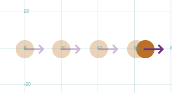
This allows students to quickly assess the behavior of the simulation without needing to spend time learning how to implement complex tools.
Easily Adjust Simulation Parameters
We have also tried to remove any coding that isn’t specifically targeted at modeling physics. For example, Tychos has a simple set of simulation parameters that can be changed with a few simple controls:
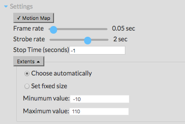
The above panel shows that a student can change the frame rate, the motion map strobe rate, set a simulation stop time, and change the extents of the viewing window – all without writing a line of code.
Coding of the GUI, rendering graphics, running the animation, etc are taken care of so there is less to program. The programs are much shorter and the code is more focused on the physics concepts, e.g calculating how force and momentum affect the position of a particle. There is no “boiler plate” code that needs to be used to get started which we have found to be cumbersome and confusing for students. Students spend less time learning programming and more time learning physics.
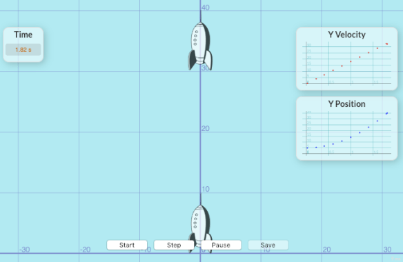
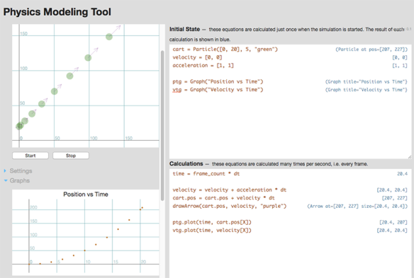
Graphing
One of the great features that we are excited about and that I have found incredibly useful in class is the built in graphing tools in Tychos. With two simple lines of code, a student can graph any variables on a simple to read graph.
This allows for the student to graph the position, velocity, and acceleration of a particle as a function of time (called motion graphs) but they can also graph energy, momentum, force, or any virtual quantity defined in the simulation code.
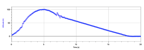
In the following example, the student has defined the kinetic energy of a particle and then has defined and displayed a graph for how the energy is changing with respect to time:
KEgraph = Graph("KE vs Time")
KE = 0.5*p.mass*p.vel*p.vel
KEgraph.plot(t, KE)
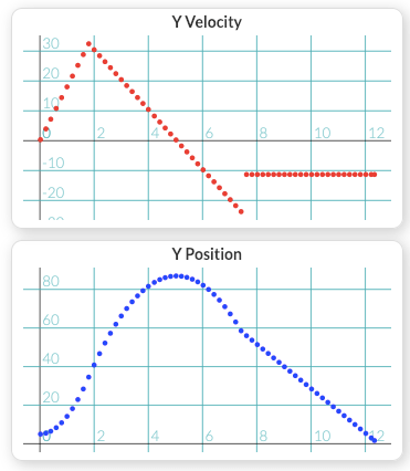
The graph then looks like this:
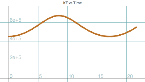
This graph appears just under the simulation window, and the student can then easily connect the behavior of the simulated particle to the behavior of the graph.
Integrated Formative Assessment:
Tychos has been built around the concept of a learning system. From the ground up, we have built in features that are designed to engage the student in the learning process. Tychos includes fast feedback in the form of instructor defined goals which are checked by the system such as “Your simulation should calculate position of particle at time 3 seconds.”

These goals keep students on track and allows for students to self assess. We have also noticed how these goals make the learning exciting. Students have expressed how much they enjoy watching the goals turn green as they accomplish them.
Teachers can also use the Goals as a quick and easy way to assess the learning progress of the entire class, and then focus on individuals that are having trouble. The teacher has the ability to peer into the individual student’s work and we are even building into the application the ability to see a “code history” of each student so that the teacher can track down the origin of a learning challenge and then direct the student to a specific solution.
Our Roadmap
We think we are off to a great start with this app, but we also realize that there are a number of great potential features that we hope to add. This is a rough outline of our future goals:
Tracking Student Progress
Soon the tool will show each student’s progress in realtime to the instructor so the instructor can maximize their time helping the students who need it. The tool will also allow instructors to see the work each student does, e.g. each attempt the student has made, the difference from the last attempt, and its outcome to help the instructor quickly deduce where the student’s thinking is and what is blocking her. Additionally, the instructor will be able to automatically export assessment data based on instructor’s defined criteria.
Custom Defined Classes
We want to give the students the ability to define reusable components so that we can further reduce the amount of code that is needed to create a simulation. We are working on some strategies to build that into Tychos.
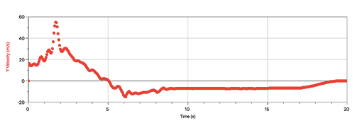
Data Export/Import
To extend the connection between Tychos experiments and in class laboratory experiments, we intend to add the ability to export and import data to and from other data collection software like Logger Pro. This will allow more precise comparisons between simulated behavior and measured behavior from motion detectors or force sensors.
Looking For Feedback
We are continuously looking for ways to improve our application, and we have no shortage of ideas. Our next challenge is finding the time and resources to make those future enhancements possible, but we are eager to have other Physics teachers try this tool out and let us know what else we should do to make this a better learning and teaching experience.
If you are interested in trying this application out, please visit our website: tychos.org. If you would like to give us feedback, or have questions, please feel free to post a comment on this blog post or contact me (stemple@srcs.org) or Winston (winston@nitidbit.com). We would love to hear from you!