Simulating Planetary Motion (Using Code!)

Simulating Newton’s Law of Universal Law of Gravity

Interactive simulations (like those created by the University of Colorado – PhET) can be really nice for impressing students, and giving them a way to explore the dynamics of a simulation. If incorporated into a lesson well, they can add to the active learning process. The question that I always struggle with though is “are the students learning how the simulation works, or are they learning how nature works?”

I have a nagging feeling that the students would possibly get more out of being able to see the simulation source code, specifically the rules of behavior of the simulation, and then through “tweaking” the code, see how those rules govern behavior. I would like to develop curriculum that would allow my students more opportunities to explore the code “behind” the simulations. This presents a few challenges that have been identified by other great physics educators, and if you are thinking about doing the same thing – I would suggest reviewing their insights. I include a quote from Ruth Chabay’s brief, but very interesting article on this topic:

To integrate computation, especially programming, into an introductory course, it is necessary to minimize the amount of non-physics related material that must be taught. To do so it is necessary to teach a minimal subset of programming constructs; employ an environment and language that are easy to learn and use; ensure that program constructs match key physics constructs; provide a structured set of scaffolded activities that introduce students to programming in the con- text of solving physics problems

This was my first attempt at doing just this, and I had some success and realized that I have some work to do.

Which Code?

A popular programming language in the Physics Modeling community is VPython. I have chosen to use a different language to use called Processing. There are reasons I chose this language, but I am sure there are reasons one would choose VPython (or other languages). At this point, I have not had the opportunity to work with VPython, so this post will not attempt to compare Processing to other languages. Perhaps I will do so in the future…

Here are some general reasons why I like Processing:

  1. It’s free and open source.
  2. Because its built on a visual programming interface, its really easy for the students to create visual content on the screen, and it is very easy to create visual animations due to the embedded “draw” loop.
  3. The official website has great examples and tutorials. It is full of great code samples and quick tutorials. You can loose yourself for hours (or days!) just having fun exploring the examples and tutorials.
  4. The IDE is simple and very similar to the Arduino IDE, so if you plan on doing any Arduino programming, the similarity is nice for the students.
  5. There is a nice vector library for doing vector operations (.add, .mult, .norm, .dot, etc.)
  6. Its object oriented so that you can have the added benefit of teaching important programming concepts – though this might be why some people might not like it.

The Simulation

The simulation that the students were introduced to was a simulation that modeled Newton’s Law of Universal Gravitation. The students were given some instructions on the basic structure of the program, and I made sure that there was some guiding comments embedded in the code. This program was inspired/adapted from a similar program created by Daniel Shiffman who has also written an amazing book on simulating nature through code called Nature of Code.

The program defines two classes. First, there is the parent class called Particle. This class defines some basic attributes like location, velocity and acceleration as well as mass. It also has some basic functions that allow it to move and allow it to respond to a force. The second class is the child class called Planet. It can do everything that a Particle can (because it inherits from the Particle class), but it can also exert an attractive force on other Planets.  Here is the code below:

/* A parent class for all moving particles
class Particle {
  PVector location;
  PVector velocity;
  PVector acceleration;
  float mass;

  Particle(float x, float y, float m) {
    mass = m;
    location = new PVector(x, y);
    velocity = new PVector(0, 0);
    acceleration = new PVector(0, 0);
  }
  
  void applyForce(PVector force) {
    // Newton’s second law at its simplest.
    PVector f = PVector.div(force,mass);
    acceleration.add(f);
  }

  void move() {
    velocity.add(acceleration);
    location.add(velocity);
    acceleration.mult(0);
  }
}

/** 
 This class defines an object that behaves like a planet.
 Planet objects extend Mover objects, so they can move. They
 also can attract other planet objects.
 **/
   
class Planet extends Particle {

  float size;
  float G = 1;

  // To create a planet, you need to supply coordinates, mass, and size
  Planet(float x, float y, float m, float s) {
    super(x, y, m);
    size = s;
  }

  // This function allows a planet to exert an attractive force on another planet.
  PVector attract(Planet p) {

    // We first have to figure out the direction of the force
    // This creates a unit vector for the direction
    PVector force = PVector.sub(this.location, p.location);
    float distance = force.mag();
    distance = constrain(distance,size + p.size,500);
    force.normalize();

    // This is where we use Newton's Law of Universal Gravitation!
    // The stength of the attraction force is proportional to the
    // product of the mass of this planet and the mass of the other planet
    // as well as the value of G. It is also inverseley proportional to
    // the distance squared.
    float strength = (G * mass * p.mass) / (distance * distance);
    
    // To get the final force vector, we need to 
    // multiply the unit vector by the scalar strength
    force.mult(strength);

    // Return the force so that it can be applied!
    return force;
  }
  
  // Just displays the planet as a circle (ellipse)
  void display() {
    stroke(255);
    fill(255, 100);
    ellipse(location.x, location.y, size/2, size/2);
  }
  
}


/** 
  This program simulates the gravitational interaction between planet objects
  **/
  
Planet planet1;
Planet planet2;

void setup() {
  background(0);
  size(800,800);
  // Inputs for each planet:
  // (x, y, mass, radius)
  planet1 = new Planet(width/2,height/4,6000,60);
  planet2 = new Planet(width/2,height/1.25,6000,60);
  
  // This is where you can change the initial velocities of the planets.
  planet1.velocity.x = 0;
  planet1.velocity.y = 0;
  planet2.velocity.x = 0;
  planet2.velocity.y = 0;
}

void draw() {
  background(0);
  
  // f1 is a force vector that is created by calling the planet's attract function
  PVector f1 = planet1.attract(planet2); 
  // Now apply that force on the other planet.
  planet2.applyForce(f1);
  // Now deal with the opposite force pair
  PVector f2 = PVector.mult(f1, -1);
  planet1.applyForce(f2);
  
  // Allow the planets to now move.
  planet1.move();
  planet2.move();
  
  // Display the planets
  planet1.display();
  planet2.display();
}

Experimenting With The Code

The students could change the initial values of the planets, such as the starting positions, the masses and radii by changing the input values of these two lines of code:

planet1 = new Planet(width/2,height/4,6000,60);
planet2 = new Planet(width/2,height/1.25,6000,60);

The planets initial velocities could also be modified by changing the values assigned in these four lines of code:

planet1.velocity.x = 0;
planet1.velocity.y = 0;
planet2.velocity.x = 0;
planet2.velocity.y = 0;

The code that actually guides the strength of the gravitational attraction between the two planets is actually very simple. This is the magnitude of the force as defined by Newton’s Law of Universal Gravity in code:

float strength = (G * mass * p.mass) / (distance * distance);

There is some slightly complicated code that controls the direction of the force and how that force is then applied to the planet object’s state of motion, but I didn’t have the time to explain this, which was a bit disappointing (see below).

For The Future

I am currently really interested in incorporating programming into the academy program, but have found myself a bit intimidated by the challenges identified by Ruth Chabay. The most significant challenge is time:

In an already full introductory physics curriculum, there is little or no time to teach major programming skills. Students who are new to programming are also new to the process of debugging; teaching debugging strategies requires even more time…Working on programming activities only once a week in a lab or recitation section may not be adequate to keep knowledge of syntax and program structure fresh in the students’ minds.

I plan on taking some time this summer to see how I could integrate computer programming more significantly into the curriculum without causing the learning of Physics to suffer – that would of course defeat the purpose!

Analyzing A Rocket’s Performance – A Common Core Assessment

Overview: What is Common? Argumentation

You might be one of the many Americans that are a bit perplexed by this whole new Common Core State Standards (CCSS) “stuff”. In this post I will try my best to explain how I designed an assessment for the first year students in the Academy that aligns with the Common Core. This was partly motivated by a district wide push to bring all curriculum in alignment with the CCSS, specifically as it relates to literacy.

For context, I will identify the educational goal that in part motivated this effort. Our school site administration has identified argumentation as a key curricular focus that all staff will address this year. This has given the school the ability to focus on literacy and has allowed the school staff to guide their efforts towards a collaborative goal.

This assessment was organized into three parts: the prediction, the analysis, and the reflection. Each part of the assessment focused on specific standards.

Part 1: The Prediction Report

If you haven’t had a chance to read a previous post where I describe how the students conducted experiments and collected data pertaining to building a predictive model, then I might suggest it, as it is really the first part of this assessment.

The standards addressed in this part of the assessment are as follows:

CCSS.ELA-Literacy.RST.11-12.3
Follow precisely a complex multistep procedure when carrying out experiments, taking measurements, or performing technical tasks; analyze the specific results based on explanations in the text.

CCSS.ELA-Literacy.RST.11-12.7
Integrate and evaluate multiple sources of information presented in diverse formats and media (e.g., quantitative data, video, multimedia) in order to address a question or solve a problem.

To summarize the first part of the assessment, the students were required to collect data in order to create a prediction report describing the performance of their model rockets. The report had to include these elements:

  1. Force diagrams (free-body diagrams) depicting the predicted forces acting on the rocket during the a) thrust phase, b) cruise phase, and c) descent phase.
  2. Net force equations that identify the causal relationship governing the motion state of the rocket.
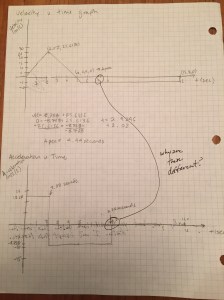
  3. Three motion graphs depicting the predicted behavior of the rocket. This included its predicted acceleration, velocity and position as a function of time.

IMG_0836

The student teams submitted these reports prior to the actual launch.

Part 2: Analysis Report

The next step was to run the actual experiment – the launching of the rockets! Although the launch day was soggy, we still had a successful afternoon, and we got some great data. The details of the launch are described in a previous post.

The standard addressed in this part of the assessment was as follows:

CCSS.ELA-Literacy.RST.11-12.9
Synthesize information from a range of sources (e.g., texts, experiments, simulations) into a coherent understanding of a process, phenomenon, or concept, resolving conflicting information when possible.

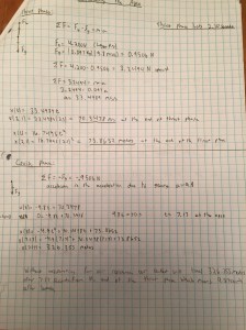
The students were given their prediction reports back, and then also given the data from the small altimeters that were used to collect altitude data. The students were then asked to create an analysis of their rocket’s performance:

IMG_0834

This report required these elements:

  1. Using the data analysis tools in LoggerPro, they had to identify:
    1. The acceleration of the rocket during the thrust phase (a best estimate)
    2. The acceleration of the rocket during the cruise phase (a best estimate)
    3. The maximum velocity of the rocket (a best estimate)
    4. The descent velocity (a best estimate)
  2. A velocity vs time graph from the information above.
  3. An acceleration vs time graph.

Part 3: Reflection (Addressing Counter-claims)

The final part of the assessment asked the students to compare the prediction and analysis reports and then propose reasons for discrepancies between the data. I also asked the students to respond to some Aristotelian counter claims by using their data and the models that we had collectively established in class.

The standards addressed in this part of the assessment were:

CCSS.ELA-Literacy.RST.11-12.8
Evaluate the hypotheses, data, analysis, and conclusions in a science or technical text, verifying the data when possible and corroborating or challenging conclusions with other sources of information.

CCSS.ELA-Literacy.WHST.9-10.1.a
Introduce precise claim(s), distinguish the claim(s) from alternate or opposing claims, and create an organization that establishes clear relationships among the claim(s), counterclaims, reasons, and evidence.

I asked the students to respond to the following questions which required that the students use data to support their analysis.

  1. Compare the predicted NET force on your rocket during the thrust phase to the actual NET force on your rocket during the thrust phase by using your data – you will need to estimate the actual NET force during this phase. Using these numbers as evidence (you must include these values in your answer), describe at least one reason these values are different.
  2. Compare the predicted maximum height of your rocket with the actual maximum by using your data. Using these numbers as evidence (you must include these values in your answer), describe at least one reason these values are different.
  3. Compare the predicted descent velocity during the descent phase to the actual descent velocity from your data. Using these numbers as evidence (you must include these values in your answer), describe at least one reason these values are different.
  4. Look at your data and then also at your prediction graphs. Describe at least two differences between the graphs, AND WHY you think these differences exist.
  5. Based on the actual data you collected, what design changes would you make IF you could create this rocket from scratch again? Give at least two examples of design changes you would make.

I also included two questions that asked the students to respond to an alternative explanation for the behavior of their rocket. These claims were specifically created in order to address student misconceptions involving inertia and residual forces.  Below I have included the questions and example student responses:

Question 1:
“Make a counter claim to the following statement from someone who is an “Aristotelian”: The reason that the rocket continued to move upwards after the fuel had run out is that the fuel force continued to push on the rocket, but lessened until the rocket reached its apex, when the rocket stopped moving and the thrust force disappeared. Once the thrust force disappeared, the rocket began falling back to earth!”

Example Response:
“This is incorrect because as soon as the fuel runs out there is no longer a thrust force acting on the rocket. After the fuel runs out the only force acting on the rocket is the force of gravity which will slow down the rocket until its velocity is zero and then the rocket will continue accelerating downward and fall to the earth.”

Question 2:
“Make a counter claim to the following statement from someone who is an “Aristotelian”:The reason that the rocket descended back to earth is because the rocket is heavier than air and so the force from gravity was greater than any air resistance force on the parachute, thus resulting in the rocket falling back to earth.”

Example Response:
“Actually, the reason the rocket descended to earth is because the forces of gravity and drag were equal. The rocket was falling at terminal velocity, and we know that when an object is traveling at a constant velocity there is no acceleration. If the force of gravity working on the rocket was greater, the rocket would be accelerating in its descent. Knowing that the rocket falls in this way, we can conclude that the forces of gravity and drag working on the parachute were equal.”

Conclusion

I am very pleased by the students’ performances on this assessment, and many of the students enjoyed the process and appreciated the opportunity to connect their learning and demonstrate their knowledge and skill. I feel that there is much to consider for the next time I do this kind of assessment, which will be at the end of the spring semester.

One area I can quickly see I need to help the students develop is making connections to data more explicit. Most students would justify their arguments by stating that a certain explanation was evident. I need to help them develop the skill of presenting evidence more clearly and then linking their arguments to the actual evidence. This was an implicit practice, but it needs to be more explicit.

I hope to hear from you all about how I might perfect this process, and prepare the students to excel on this kind of authentic, problem based assessment.

Thanks!

We Have Lift Off!

15414703973_b0258a08ca_h  15846865828_b08d8515cd_h 16033503742_be978fd9ca_h

This is a follow up post to Modeling A Rocket’s Journey – A Synthesis where I described how the students in the first year program were engaged in creating a predictive report for their model rockets. I want to emphasize that these model rockets were not kits. Each rocket was designed using 3D CAD software, and each component was either fabricated from raw material, or was created from material that was not intended for use in model rocketry. The only exception to this is the actual rocket motor.

The next step was to launch the rockets and have the altimeter payload collect altitude data.

Launch Conditions – A Bit Soggy

Unfortunately the week of our scheduled launch happened to be a week of some pretty hefty rains. We rescheduled the launch twice before finally accepting the soggy launch conditions. With umbrellas and rain jackets, we trudged out to the baseball diamond and got to work setting up for the launch. We had some minor difficulties in the wet weather, but eventually had a very successful launch day.

Most of the rockets were able to launch and deploy their valuable payload – the Pnut Altimeter.

15414689283_8197c70584_h

The students seemed very excited to finally see the rockets launch, and to see the successful deployment of the parachutes. Although we all got a little wet and muddy, we had a great time!

The Altimeter Data

The altimeters use a small barometric pressure sensor to collect altitude data (the altimeters also contain a small temperature sensor and voltage sensor). The altitude is recorded in feet every .05 seconds. Here is an example of one rocket’s recorded flight data:

altitude_vs_time

https://plot.ly/~stemples/9

The students were then asked to use the data to create a comparative analysis report. I will detail how the assignment was set up and also discuss how the students performed on this assignment. That will be for another post.

I want to also thank Mr. Kainz for his amazing photos that are displayed here.