Modeling A Physical Pendulum – Another Adventure in Coding Nature

Rotational Dynamics Are Difficult to Learn… and to Teach

One of the most difficult units for AP Physics students is rotational mechanics. It can also be one of the hardest to teach. With that said, I really like rotational mechanics, but I want my students to enjoy it more. I want them not be be bogged down in some of the more difficult theoretical aspects of the rotational motion. There are several reasons for this topic being challenging I think – the use of the polar coordinate system, the introduction to the concept of a distribution of mass as opposed to just thinking about objects as point particles, the cross product of vectors producing a result pointing in the Z axis…yikes, it can get pretty heavy.

As a teacher, it is also tricky to come up with good investigations that allow students the opportunity to explore rotational dynamics. They do exist, and some are really good, but I also think that many don’t exactly build a strong link between the conceptual and mathematical models. Rolling a ring and a disk and sphere down a ramp can be a great demonstration that things that roll certainly do not behave like blocks or carts moving down a ramp, but its hard for the students to explore further – to build a predictive model that is mathematically precise. The normal way of things is to jump into the math and reveal the underlying mechanics through fairly complex derivations.

Simulating The Angular Momentum Principle

This year I decided to turn to a computational approach. I wanted the students to computationally experiment and discover the fundamentals of rotational mechanics. In order to do this, we started from the Angular Momentum Principle. This is the approach used in the wonderful textbook Matter and Interactions:

Στ ·Δt = I·Δω

The idea here is simply that a torque acting on an object (that is free to rotate around a pivot point) for a specified amount of time is going to cause an object to experience a change in its rate of spinning – called its rotational velocity.

Simulating A Physical Pendulum

Having the students start with this principle, they could learn some interesting mechanics of rotating bodies by building a simulation of a physical pendulum. A simple pendulum is “simple” in that it represents a single point mass hanging on a massless string. A physical pendulum has physical dimension, and so the body has to be modeled as having a distribution of mass. This gets really tricky to analytically model – especially the time dependent functions describing its motion.

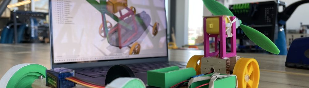
But with a computational approach students could easily apply the momentum principle frame by frame. The students in my class were able to create a simulation of a physical pendulum in just over one class period. The pendulum that they modeled was a bar with weights at either end. The weights had different masses so that the bar would swing.

https://tychos.org/scenarios/250

The students set about building their simulations in Tychos – a web based simulation builder. As the students coded the simulation, they were continuously engaged in discussions about the mechanics of the code and the mechanics of nature. I asked the students to change the masses, or change the length of the bar, or the mass of the bar. They would run their simulations and discover that something didn’t quite match what they thought should happen. Students would then look for errors in the code, or they would question their own assumptions about the physics involved.

When they finished their simulations, and they were confident that their simulations were working, I had the students then use the simulation to investigate the energy of the rotating system. After some discussions about the transference of energy from the gravitational field to the kinetic energy (rotational) of the bar and the weights, the students discovered that their simulations also seemed to model the conservation of energy.

We didn’t stop there though. We had to see if the simulation did indeed match reality. This is called deployment in the modeling pedagogy. Using a meter stick, some disks that I had made for an earlier investigation, and a Vernier rotational sensor, I constructed a real physical pendulum.

To test the simulation, students were asked to identify all the inputs that would need to be measured and then entered them into their simulations. The students then used the conservation of energy to calculate rotational speed of the bar when the bar was released from an angle of 60 degrees – with the heavier weight above the lighter weight.

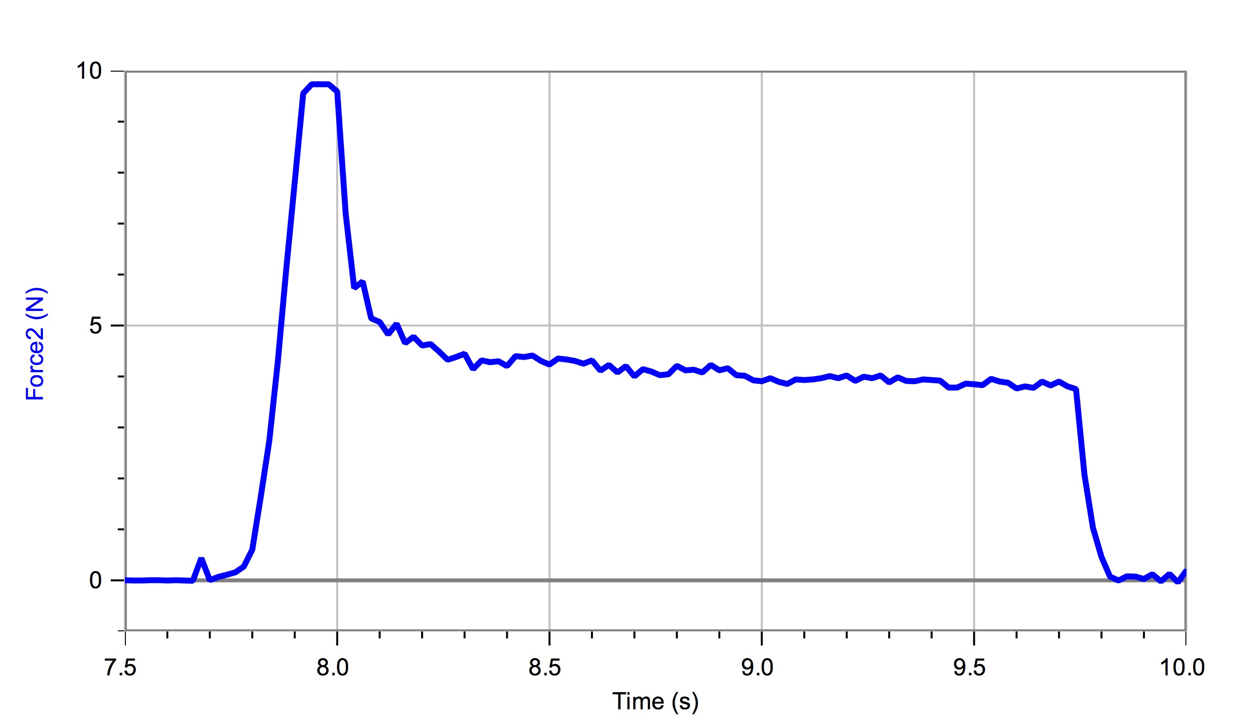
The students calculated a final rotational velocity of 2.8 radians/second. We then ran our test and graphed the angle of the bar as well as the rotational velocity of the bar (see graphs below). They measured a rotational max velocity of about 2.6 radians/second. The students were pretty satisfied with this result.

omega_graph

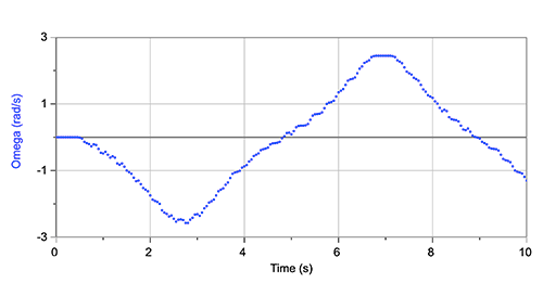
angular velocity of the bar

theta_graph

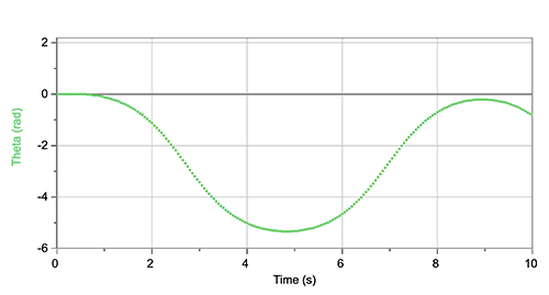
angular position of the bar

I then had the students graph the results of their simulations, and it was quite satisfying to see that the simulations and the sensor readings were matching really well.

sim_phys_pendulum

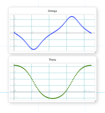
graphs produced in Tychos

This led to some more interesting discussions around simulating axel friction and air resistance. We also discussed the shapes of the graphs and what might be going on with their mathematical structure. This was far more interesting than just having them read out of a textbook and then solve some problems on paper, and my guess is that the students gained an understanding of the physical mechanics by having to debug their own simulated mechanics. They were able to investigate errors in their own code, but by doing so, see how the position of the weights, and the masses and the angle changed the behavior of the simulation and the motion graphs. I think the students also really enjoyed this approach, and based on how they were talking about their simulations and the experiment, they demonstrated to me that they had grasped a deeper understanding of rotational mechanics.


Building the Electrical Current Model with The Amazing $25 Programmable Power Supply

Not Just For Teaching Robotics

Thanks to the generous donations of supporters of the Physics Academy, we were able to purchase a new set of Arduino Uno micro-controllers for use in this year’s robotics competition. As I was planning out the unit on teaching DC circuits, I realized that some of our DC power supplies might need to be replaced. I got to thinking – could the Arduino replace these hulking, expensive power supplies?

product.exps._hero.001.590.332

The answer has been (with one caveat) – yes. The above power supplies are nice, no doubt about it, but they are big, costly ($199) and they are not as nearly as extensible as a micro-controller.

Arduino_Uno_-_R3

The Arduino micro-controller can act as a fixed 5V power supply, or using its PWM pins, you can vary the voltage from 0V to 5V with a resolution of about 20 mV. The other advantage about using the Arduino is that it gives you a chance to teach a little bit of programming too! In our case, it allows for a great introduction to robotics well before we are ready to start our unit on robotics.

The one disadvantage is that you can’t test any circuits that need over 5V of electrical potential difference, nor can you test things like motors or other higher current (> 40 mA) circuits. We didn’t find this to be a big problem, but if you do, you can actually purchase a shield (an attachment that fits on top of the Arduino) from Adafruit Industries that allows you to use a higher voltage, higher current power supply that is controllable through the Arduino.

Mapping Electrical Potential (Voltage)

One of the first activities that the students do, which is a great activity from the AMTA curriculum repository, is to have the students “map” the voltage between two metal bars that are partially submerged in water.

IMG_1870

Using the Arduino as the power supply, the students use a multimeter to check the voltage at specific locations on a grid that is placed under the transparent pan holding the water. These numbers are recorded into a spreadsheet. Excel has a great tool for doing a 3D map of the values.

potentialmap

What results is a really nice visualization of the potential isolines and the spacial variance of the voltage, and thus the electrical field.

Ohm’s Law – A Flow Model

We then move from voltage maps to flow model. The students investigate how voltage, current and resistance are related to one another. The students begin by investigating the current flowing into and out of a resistor, and most are surprised to find that the current in the same flowing into a resistor as it is flowing out. They expect that current should be “used up” by the resistor – causing a bulb to glow for example. When they find that this is not the case, they either think that they have done the experiment incorrectly or that perhaps the multimeter is not precise enough. This confusion comes from the idea that they are expecting current and energy to be equivalent.

IMG_1918

The hydrology analogy is introduced as a possible model for describing this phenomenon. We discuss the movement of water past a water wheel, and how the water flowing into the wheel is equal to the amount of water flowing “out” from the wheel. Students quickly realize that the wheel still turns, not because the water is “used up”, but because the water looses energy.

The final challenge for the students is to confront the oddity that is parallel circuits. This is made a bit easier by thinking about the flow model, but the confusion with parallel circuits stems from the idea that a battery is a constant current supplier – which of course it is not. The Arduino, just like a battery, will increase the amount of current flowing from its digital output pins when more pathways are added for the current to flow. This is where I would be careful to make sure however that you don’t approach the 40 mA limit. If you do, you can get some weird results in your observations as the Arduino will naturally cut off current draws around this range to protect its electronics.

Conclusion

The switch to the Arduino has been quite successful, and as stated before, it launches the students into the robotics project with a knowledge that the Arduino is simply a controllable power supply. They learn very quickly from that point on that the Arduino can also act like a voltmeter too! Using its analog input and switching the digital pins to be input pins, the Arduino can also mimic the functionality of a multimeter. If you are considering new power supplies, I would recommend looking into this as an option.

Simulating Planetary Motion (Using Code!)

Simulating Newton’s Law of Universal Law of Gravity

Interactive simulations (like those created by the University of Colorado – PhET) can be really nice for impressing students, and giving them a way to explore the dynamics of a simulation. If incorporated into a lesson well, they can add to the active learning process. The question that I always struggle with though is “are the students learning how the simulation works, or are they learning how nature works?”

I have a nagging feeling that the students would possibly get more out of being able to see the simulation source code, specifically the rules of behavior of the simulation, and then through “tweaking” the code, see how those rules govern behavior. I would like to develop curriculum that would allow my students more opportunities to explore the code “behind” the simulations. This presents a few challenges that have been identified by other great physics educators, and if you are thinking about doing the same thing – I would suggest reviewing their insights. I include a quote from Ruth Chabay’s brief, but very interesting article on this topic:

To integrate computation, especially programming, into an introductory course, it is necessary to minimize the amount of non-physics related material that must be taught. To do so it is necessary to teach a minimal subset of programming constructs; employ an environment and language that are easy to learn and use; ensure that program constructs match key physics constructs; provide a structured set of scaffolded activities that introduce students to programming in the con- text of solving physics problems

This was my first attempt at doing just this, and I had some success and realized that I have some work to do.

Which Code?

A popular programming language in the Physics Modeling community is VPython. I have chosen to use a different language to use called Processing. There are reasons I chose this language, but I am sure there are reasons one would choose VPython (or other languages). At this point, I have not had the opportunity to work with VPython, so this post will not attempt to compare Processing to other languages. Perhaps I will do so in the future…

Here are some general reasons why I like Processing:

  1. It’s free and open source.
  2. Because its built on a visual programming interface, its really easy for the students to create visual content on the screen, and it is very easy to create visual animations due to the embedded “draw” loop.
  3. The official website has great examples and tutorials. It is full of great code samples and quick tutorials. You can loose yourself for hours (or days!) just having fun exploring the examples and tutorials.
  4. The IDE is simple and very similar to the Arduino IDE, so if you plan on doing any Arduino programming, the similarity is nice for the students.
  5. There is a nice vector library for doing vector operations (.add, .mult, .norm, .dot, etc.)
  6. Its object oriented so that you can have the added benefit of teaching important programming concepts – though this might be why some people might not like it.

The Simulation

The simulation that the students were introduced to was a simulation that modeled Newton’s Law of Universal Gravitation. The students were given some instructions on the basic structure of the program, and I made sure that there was some guiding comments embedded in the code. This program was inspired/adapted from a similar program created by Daniel Shiffman who has also written an amazing book on simulating nature through code called Nature of Code.

The program defines two classes. First, there is the parent class called Particle. This class defines some basic attributes like location, velocity and acceleration as well as mass. It also has some basic functions that allow it to move and allow it to respond to a force. The second class is the child class called Planet. It can do everything that a Particle can (because it inherits from the Particle class), but it can also exert an attractive force on other Planets.  Here is the code below:

/* A parent class for all moving particles
class Particle {
  PVector location;
  PVector velocity;
  PVector acceleration;
  float mass;

  Particle(float x, float y, float m) {
    mass = m;
    location = new PVector(x, y);
    velocity = new PVector(0, 0);
    acceleration = new PVector(0, 0);
  }
  
  void applyForce(PVector force) {
    // Newton’s second law at its simplest.
    PVector f = PVector.div(force,mass);
    acceleration.add(f);
  }

  void move() {
    velocity.add(acceleration);
    location.add(velocity);
    acceleration.mult(0);
  }
}

/** 
 This class defines an object that behaves like a planet.
 Planet objects extend Mover objects, so they can move. They
 also can attract other planet objects.
 **/
   
class Planet extends Particle {

  float size;
  float G = 1;

  // To create a planet, you need to supply coordinates, mass, and size
  Planet(float x, float y, float m, float s) {
    super(x, y, m);
    size = s;
  }

  // This function allows a planet to exert an attractive force on another planet.
  PVector attract(Planet p) {

    // We first have to figure out the direction of the force
    // This creates a unit vector for the direction
    PVector force = PVector.sub(this.location, p.location);
    float distance = force.mag();
    distance = constrain(distance,size + p.size,500);
    force.normalize();

    // This is where we use Newton's Law of Universal Gravitation!
    // The stength of the attraction force is proportional to the
    // product of the mass of this planet and the mass of the other planet
    // as well as the value of G. It is also inverseley proportional to
    // the distance squared.
    float strength = (G * mass * p.mass) / (distance * distance);
    
    // To get the final force vector, we need to 
    // multiply the unit vector by the scalar strength
    force.mult(strength);

    // Return the force so that it can be applied!
    return force;
  }
  
  // Just displays the planet as a circle (ellipse)
  void display() {
    stroke(255);
    fill(255, 100);
    ellipse(location.x, location.y, size/2, size/2);
  }
  
}


/** 
  This program simulates the gravitational interaction between planet objects
  **/
  
Planet planet1;
Planet planet2;

void setup() {
  background(0);
  size(800,800);
  // Inputs for each planet:
  // (x, y, mass, radius)
  planet1 = new Planet(width/2,height/4,6000,60);
  planet2 = new Planet(width/2,height/1.25,6000,60);
  
  // This is where you can change the initial velocities of the planets.
  planet1.velocity.x = 0;
  planet1.velocity.y = 0;
  planet2.velocity.x = 0;
  planet2.velocity.y = 0;
}

void draw() {
  background(0);
  
  // f1 is a force vector that is created by calling the planet's attract function
  PVector f1 = planet1.attract(planet2); 
  // Now apply that force on the other planet.
  planet2.applyForce(f1);
  // Now deal with the opposite force pair
  PVector f2 = PVector.mult(f1, -1);
  planet1.applyForce(f2);
  
  // Allow the planets to now move.
  planet1.move();
  planet2.move();
  
  // Display the planets
  planet1.display();
  planet2.display();
}

Experimenting With The Code

The students could change the initial values of the planets, such as the starting positions, the masses and radii by changing the input values of these two lines of code:

planet1 = new Planet(width/2,height/4,6000,60);
planet2 = new Planet(width/2,height/1.25,6000,60);

The planets initial velocities could also be modified by changing the values assigned in these four lines of code:

planet1.velocity.x = 0;
planet1.velocity.y = 0;
planet2.velocity.x = 0;
planet2.velocity.y = 0;

The code that actually guides the strength of the gravitational attraction between the two planets is actually very simple. This is the magnitude of the force as defined by Newton’s Law of Universal Gravity in code:

float strength = (G * mass * p.mass) / (distance * distance);

There is some slightly complicated code that controls the direction of the force and how that force is then applied to the planet object’s state of motion, but I didn’t have the time to explain this, which was a bit disappointing (see below).

For The Future

I am currently really interested in incorporating programming into the academy program, but have found myself a bit intimidated by the challenges identified by Ruth Chabay. The most significant challenge is time:

In an already full introductory physics curriculum, there is little or no time to teach major programming skills. Students who are new to programming are also new to the process of debugging; teaching debugging strategies requires even more time…Working on programming activities only once a week in a lab or recitation section may not be adequate to keep knowledge of syntax and program structure fresh in the students’ minds.

I plan on taking some time this summer to see how I could integrate computer programming more significantly into the curriculum without causing the learning of Physics to suffer – that would of course defeat the purpose!

Modeling A Rocket’s Journey – A Synthesis

A Synthesis Of All The Models (Thus Far)

In this post I will describe a culminating activity for the first year students in the Academy. This is really the destination that the students have been headed towards since the beginning of the course. Everything they have learned is synthesized in this activity where the students gather data from various observations/experiments and then use the data to predict their own model rocket’s journey.

Note: There were two significant simplifications that we had to make based on the ability level of the students and the physics content covered in class. We had to assume that there was no air resistance force acting on the rocket during the thrust and cruise phases. We also assumed that the mass of the rocket did not change. I intend to have the students reflect on how this might affect the predictions and then analyze the actual performance data. More on this later…

Measuring The Rocket Engine Thrust

We first needed to figure out the average force exerted by the rocket motor on the rockets and the time interval during which that force would be applied. This would give the students both the thrust force and the length of time of the thrust phase. We needed to collect force measurements for the rocket motors that we were using (C6-5). You can actually download this from many different websites, but it was much more fun to actually do it ourselves! Mr. Holt made a neat little rocket motor holder that was attached to a force meter and we went out into the rain to test the motor (see video below – thank’s Gary!):

The force data was then shared out to the students – here is what the graph looked like:

rocket-engine-test

And this is the force vs time graph one retailer posted on their website:

Although the students had not been introduced to the concept of Impulse-Momentum transfer, we can use the average force, and that seems to work out really well. Just to make sure we could do this, I used the Integral tool in LoggerPro to measure the impulse, and it came out to 8.83 N s – really close to what Estes states – 8.8 N s.

A Mini Wind Tunnel Test

The students then needed to measure the drag force on their parachutes (all cut on our new laser cutter) as a function of air speed so that they could estimate the terminal velocity of their rocket during the descent phase.  Next step was to test the parachutes. Luckily, Mr. Holt and I had helped two of our previous students create a really nice wind tunnel. We used a force meter attached to a vertical post inside the tunnel…

parachute_test

…and then we used a little Kestrel anemometer to measure the air speed…

air_speed

Students were able to increase the air speed in the tunnel by turning a rheostat that controlled the fan speed. They then measured the wind velocity and graphed that against the measured force – just like NASA!

Here is some sample data to show how the results came out – not bad!

parachute-test-data

Students now had a way to estimate the descent velocity because they could calculate the gravitational force on their rocket, using the measured mass of their rockets, and then they could use their data to find the corresponding wind speed.

Putting It All Together

As part of their final (50%), the students were asked to then take this data, measure the mass of their model rocket and construct a prediction. The prediction was to include these five elements:

  1. A set of force diagrams for the different phases – thrust, cruise, and descent. The diagrams also had to include accompanying net force equations.
  2. An acceleration vs time graph.
  3. A velocity vs time graph.
  4. A position vs time graph.
  5. Finally a calculation sheet that includes all calculations required to create the motion graphs.

The students have been asked to turn this in before the actual launch.

As we collected the data above, I never explicitly reveal how the data should be used to make these predictions, but I do give them some guiding questions that orients them. They work with their partner’s on this report, but I warn them that they will both be held responsible for understanding the process of creating the prediction report.

Testing the Predictions

Each student rocket will be equipped with a small altimeter (from Apogee Rocketry – love this thing!).

This altimeter records altitude data in 1/10 of a second intervals, and we have found it to be very accurate and reliable. We will be launching next week, so tune in soon for an exciting update on how the launches went!

Building The Net Torque Model – Part 3

Appending The Conservative Models

After investigating the causal relationship between torque and angular acceleration, I introduced the possibility to the class that perhaps we also needed to revisit the Energy Transfer Model and the Momentum Transfer Model. The students agreed that an object that is rotating must have energy. This was pretty easy to demonstrate.

I set up a situation in the class where two of the variable inertia disks that we created on the 3D printers were placed at the top of an inclined ramp. The internal marbles were placed at two different configurations inside the disks and then the students predicted which disk would reach the end of the ramp first. I was pleased to find out that the class appeared to agree that the disk with the marbles located closer to the radius would be the winner. I really think that our investigation with the variable inertia disks solidified the students’ conceptual understanding of rotational inertia and the importance of mass distribution.

I have not yet found a good experiment where students could discover the rotational kinetic energy relationship, so I decided to take them through a derivation based on linear kinetic energy. I then asked the students to do some whiteboard work. I asked them to demonstrate that the disks would indeed reach the end of the ramp at different times. Although this wasn’t strictly a constructivist approach, it was good practice in doing some fairly difficult algebra without numerical values – something the students traditionally are not very good at.

We then moved onto momentum. Again, I started by reviewing the Momentum Transfer Model for a particle. At this point the pattern had been fairly well established. The relationship between angular and linear quantities seemed to have taken hold because the students were quick to propose a mathematical definition for angular momentum. Our next goal was to figure out whether this was a conserved quantity.

Mr Holt and I had created a set of metal disks that could be attached to the rotary sensors. I decided to create our own, rather than (sorry Vernier) buy them as I thought that the commercial kit was over priced. It wasn’t too hard to create the disks, especially when you have access to a CNC plasma cutter!

image1

The students attached one disk to the rotary motion sensor and then got that disk spinning. They then took a second disk that had small magnets attached to it, and dropped this disk onto the spinning disk. The students compared the angular velocity before and after the disks were combined and then calculated the angular momentum of the system before and after. The data we got was quite good with the class getting in the range of only about a 5% to 6% difference.

Wrapping it Up (or Un-Rolling It Down)

As a final deployment, I decided to try the deployment activity that Frank Nochese did with his students. It seemed like a good (and fun) way to wrap up our model (or as I have already argued – models).

Before doing the deployment activity, I reviewed all the model specifics with the students. My point here was to impress on them that what we had not really built a new model, but rather had extended many of the prior particle models to include rigid extended bodies. This generally only required that we consider the moment arm in all the particle models. I think this really helped a number of students see the connection between models that they felt they understood and all this rotational stuff that seemed a bit confusing.

I then set them up with the deployment activity, but I asked them to specifically solve the problem using both energy and net torque. There was some success, but I realized that the task was a bit much for the class. Once again, it is clear that I need to give them more practice with these problems that require multiple steps and that involve algebraic manipulation of symbols without numbers. Plenty of time to practice that!