Investigating Velocity vs Time Graphs

photo

Investigating An Object’s Velocity Graphically

The first year students began this week to investigate velocity vs time graphs for moving objects. I start the Constant Acceleration Particle Model by having the students analyze these graphs first. This is a bit different than how I used to do this, but I think it works better because it allows the students to make several observations about an object whose velocity is changing and it introduces an interesting new way to see graphs of rates vs time.

First, the students repeat the constant velocity investigation with the buggies, but this time we look at the velocity vs time graph created by LoggerPro. They see that the velocity is not perfectly constant, but that the average velocity is very close to the slope of the position vs time graph. This once again validates our understanding of the slope as being the average velocity.

What Does The Integral Button Do?

Without explaining anything about what that “Integral” button does in LoggerPro, I ask the students to simply give it a try. They see that the area under the graph is filled in with a solid color. I point out that LoggerPro associates a numerical value to this area. I ask the students to look closely at the units.

They get a bit confused with “s*m/s”, but that allows me to strengthen their understanding of how dimensional analysis works. Eventually everyone in the room agrees that this reduces to just meters. So the next question is “what meters?” What is this a measurement of?

They immediately suggest that it might be how far the buggy traveled in this time. The students check this and with a high degree of accuracy, it appears that this is indeed what the area represents! Cool, a new way to look at graphs.

From Rectangles to Triangles

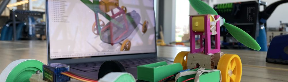
The next step is to move onto an object that is accelerating at a constant rate. The students use the motion detectors to now look at a cart being pulled by a small weight that is attached to a string – what is called a “modified Atwood’s machine”. After collecting the velocity data and graphing it, the students once again use the linear regression tool to find the slope of this graph.

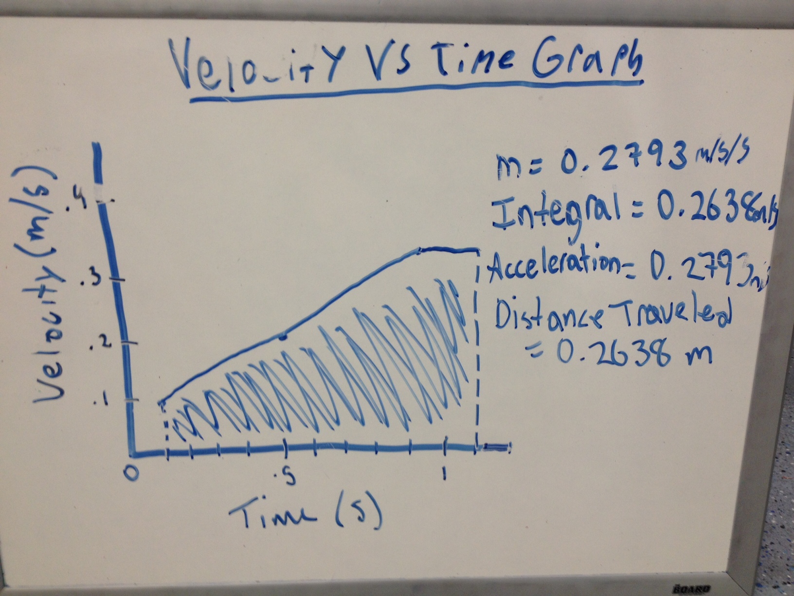
This allows us to discuss what the slope of this graph represents. Once again we get into a discussion of units because the units identified on the graph are m/s/s. The students see that this slope is actually describing the rate at which another rate (velocity) is changing.

We then use the integral tool again for the case of an accelerating cart, and it appears to work really well (see the above picture). Students share out on their whiteboards the graphs they observe, with the slope and integral value identified. The class seems pretty convinced that these quantities represent the characteristics of the observed phenomenon, so we are off to our first deployment…


Deploying The Constant Velocity Particle Model

photo

Proof is In The Deployment (Prediction)

This week the first year Academy students put their knowledge to the test. One of the key elements of the modeling pedagogy is that students are given a chance to test their predictive powers using the model that they have built. This stage of the modeling cycle is called deployment. When a model is deployed, the students describe, represent and most importantly predict the behavior of a situation they have not previously encountered.

In this case, the model the students were deploying is the constant velocity particle model. This analytical model describes, represents and predicts the behavior of a particle moving at a constant velocity. For the past few weeks, students have been building the model, informed through experimentation/observation and some guidance from staff.

In this deployment activity, students were asked to predict the location where two constant velocity buggies would collide. The two buggies had different velocities and were separated a distance of 1.2 meters. The students were asked to describe, represent and quantitatively determine the position where the two buggies would collide.

The students seemed to be satisfied with the results, and so next stop…the constant acceleration particle model.

First Year Students Begin Learning About Constant Velocity Particles

photo

And The White Boarding Begins

We are off to a great start with our new students. They did an exceptional job tackling our first observational “lab” (the Buggy Lab without motion detectors), and they got the hang of white boarding pretty quickly. As can be expected, some students were very quiet, but many participated in the group discussion, and everyone was engaged with their individual groups.

One thing discovered by the students was how important it is to draw your graph axis scale correctly. Some of the graphs created were not linear due to the fact that students tried to “squeeze” points onto the graph by effectively warping the axis. This was a good learning opportunity and I explained that in the future we would first be creating our graphs on a computer and that they were to translate the shape and not be too concerned with precisely placing their points according to the imprecisely drawn graph axis.

This also brought up the point made by one student whose team had created a graph that looked like the buggy had gone backward in time! This prompted some great discussions about time and position, but more importantly it allowed me to ask the students if it made sense to “connect the dots” on their graph. A student perceptively commented that it didn’t really make sense because it gave the impression that all the data had been gathered in one trial. We then identified that a better way to show that each data point represented a different trial would be to NOT connect them. Nice work class.