Simulating Circular Motion: An Inquiry Approach

This semester I have been very busy working on a new approach to teaching Physics. This has actually been part of an effort that has spanned more than three years, but this year I have really embraced this change and I have much to share.

This post is a preview of many to come. I am going to write several posts documenting my efforts and experiences throughout the school year. Hopefully these posts will help me capture what I have learned in the process, and perhaps will be a guide for anyone else who might be interested.

Analytical Models Emerge From Computational Models

With the help and insights of others, I have been mapping out a new scope and sequence for teaching Physics that incorporates computational modeling as the primary method of modeling Physics. Rather than looking at computational modeling as an “add on”, I have been exploring the idea that analytical models are emergent. Computational models are more fundamental and analytical models emerge from those computational models.

The basic approach here has been to start with computational modeling, and then to allow the students to discover the analytical models that are revealed. This has been an exciting “unveiling” of physical patterns for the students. The other thing that I have witnessed is that students seem to intuit the principles of Calculus, even though my students are not at that level in mathematics training. More on this in a future post.

In future posts, I will report out on how this has been going and what I have learned in the process. For now, I simply want to share an example.

The Inquiry Lessons: Discovering Centripetal Acceleration

One of the aspects of this project has been to re-invent many of my lessons. I have been creating inquiry based lessons based on an approach known as POGIL. I am not POGIL trained, so I wouldn’t say my activities are actual POGIL activities – they are POGIL “inspired”.

In the first lesson, students learned how to simulate an object moving in a circular path. I have attempted to incorporate an inquiry approach where students are guided using questions, as opposed to holding their hands. This approach can be messy, but I have found it has always lead to great conversations, unanticipated insights from the students and it gives the students a sense of discovery.

I have included a link to the lesson which you are free to copy, modify, etc. without any restrictions.

Lesson 1: Simulating Spinning Motion

Keep in mind that my students had already learned how to code movement, so if you are new to computational modeling, I will soon be writing some posts that introduce students to this approach and to computational modeling in general.

In the second lesson, students simulated circular motion using angular quantities. They then explored how they could represent the tangential velocity and then they explored what the acceleration was. This led them to discover that the simulation revealed that the acceleration vector pointed to the center of the circle. Through some guided inquiry, they discovered a number of interesting details, such as the acceleration increased when the radius declined, and that the tangential speed had a significant affect on the acceleration.

Here is a link to the lesson:

Lesson 2: Circular Motion

I do use a tool, that I am actually partly developing with some friends as the simulation software, called Tychos, but you can modify the lesson to use any coding platform you like (of course I like Tychos, but I am a bit biased!)

Please feel free to comment here to give me feedback on the lessons if you feel inclined. I am certainly on a learning path myself, and I am sure there are many improvements that could be made!

Thanks in advance,

Steve.


The Great (Mini) Robot Race

Robotics – The Synthesis Project

The final project of the two year academy program requires that the students design, fabricate, program and test an autonomous robot. We have been doing this project since the inception of the program, but this year we have made some significant improvements on the project. In this post I will explain the project, and highlight those improvements.

This project is an extremely challenging task that requires successfully completing several “sub-projects”. We tell the students at the beginning of the school year, that this project is more difficult than any of the other projects – by a long shot!

“If you haven’t done everything, then you haven’t done a thing.” – Red Whittaker

We completely changed our robot competition parameters this year. In previous years we had the students design sumo wrestling battle bots. Although this was a fun project, we started to notice that some robots performed really well without really having to “think”. These robots generally lumbered around the ring, sometimes without even actually “seeing” their opponents. Through pure luck they just managed to push their lighter opponents out of the ring. We decided that we needed to change the project in order to force teams to be smarter and we also wanted to get away from a robot competition that seemed to focus on aggressive battle.

Ironically, I suppose, our robot project changes were inspired by the classic Nova film that documented the DARPA challenge known as the Great Robot Race. In this race, the autonomous vehicles raced through the Mohave dessert on a course that was revealed to the competitors only hours before the beginning of the race.

Bob set about building an impressive “maze” for the robots to navigate. The robots had to make their way through a series of 90 degree turns defined by a series of connecting corridors with vertical walls about 20 cm tall. The robots were then given two attempts to make it through the course as fast as they could.

The Brains and Braun

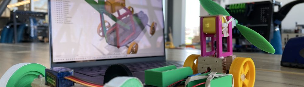
When we first started this project about twelve years ago, we first used a Java based board that we liked, but it was really expensive and we didn’t really need much of the hardware and software features that it offered. About eight years ago, the Arduino board was taking the Maker community by storm and we decided to hop on the Arduino bandwagon, and we have been very happy ever since. The simplicity, online community, the plethora of code examples and tutorials as well as the price have been key points in why we have decided to keep using the Arduino. This year we decided to incorporate DC motors from Sparkfun and Adafruit’s motor shield. The combination allowed the students more flexibility regarding drive train design, and also allowed for some interesting discussions around the advantages and disadvantages of servos vs dc motors. Our only complaint with the shield would be that it would be nice to have the headers pre soldered!

Designing The Circuitry

fritzing-preview-pcb

One of the major additions to the project was to require that students design and fabricate the circuitry for their robots. We did this by introducing two new skills to the project. Students had to learn how to use a printed circuit board (PCB) design software known as Fritzing, and then they had to learn how to fabricate their PCB boards using a CNC mill.

There are a number of amazing PCB design tools out there – and many are free! They all have their strengths and weaknesses. Here is what we found out as we did our research to find the right tool.

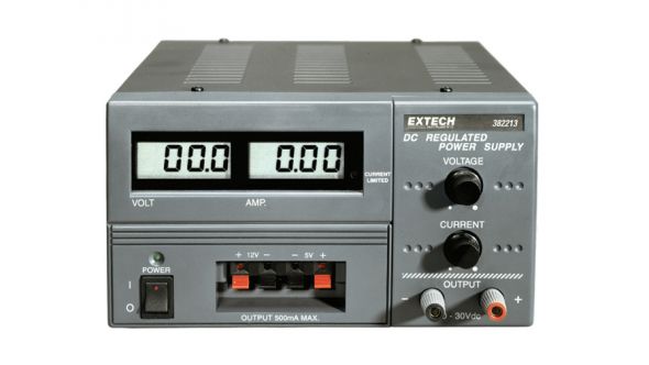
Autodesk’s Circuits is great because its web based, super easy to use and has an amazing feature where you can actually simulate the circuit. You can add a virtual voltmeter of ammeter to your virtual circuit and then with a push of a button, you can get virtual readings on the meters. I found this tool to be amazing for teaching circuitry and I allowed the students to use it as a “key” for their worksheets. It also has the ability to simulate an Arduino too! You can add an Arduino to your project, connect up LED’s, servos, etc. and actually see them light up or rotate as you change the code. It is a bit limited in that it doesn’t support most added libraries, but it is still amazing. We eventually decided not to use it for PCB design because it is unfortunately a bit clunky and doesn’t allow for much customization of the board.

Eagle is of course one of the most advanced and feature rich PCB design tools out there. It is also very complicated. IT of course offers the largest toolset, complete control of the design process and the free version is as close to a professional tool as one could hope for. The problem is that all these features come at a price – complexity. If we had an entire year to spend on this project, I might have decided to go with this tool, but we needed something that the students could learn quickly and weren’t going to get frustrated with…

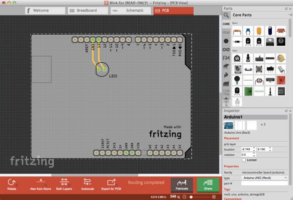
Fritzing is a free, open source “beta” software that is very similar in look and feel to Autodesk’s Circuits – in fact I think Autodesk’s product must have been inspired by Fritzing? Although Fritzing lacks the amazing simulation tools that Autodesk Circuits has, it does offer a much better PCB design environment. The options that are available for editing the component foot prints, the PCB attributes, etc. make it really nice to work without making the tool too complex. This is the tool we decided to teach and use in class, and the students liked it.

pcb-milling-opener

Fabricating The Circuitry

Back in the fall we decided to invest in a small CNC mill produced by a local company out of San Francisco named Other Machine Co. This machine, called the OtherMill has been an amazing addition to the lab. With this machine, we have been able to teach the students how to fabricate their own PCB’s. The OtherMill is not just for PCB fabrication, in fact we have used it to mill small aluminum parts as well.

2323-00

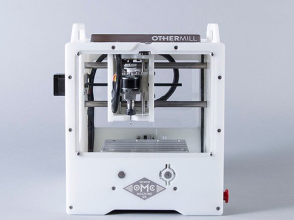
This micro CNC desktop mill is super easy to setup, really easy to use and plays really nicely with Fusion 360 – our 3D CAD and CAM software. I was incredibly surprised and pleased by how easy it is to learn the operating software – known as OtherPlan. The company has a great support website full of great tutorials, and we were able to teach all the students how to use the machine in just a few days.

The PCB files generated by Fritzing (we exported them as Gerber files) worked flawlessly with the OtherMill, and within a very short period of time, all the students had designed and fabricated single sided PCB boards for their robots.

img_3283

The Final Results

As with any major changes to a project, there are lessons to be learned. We realized that the task was rather complicated and many of the students did not make it as far through the course as they had hoped. It was clear however that this competition proved more interesting from the perspective of getting students to see the importance of software design. Not only did we see very different software strategies, but the variance in hardware design was surprising. They really had to think about how the hardware and software had to work together, and they had to think about optimization. This was a clear advantage of this competition over the previous year’s competitions. Students spent far more time trying to figure out how they were going to shave time off their attempts, and how they were going to adjust software and hardware to better navigate the course. From our perspective, the changes to the project proved to be fantastic, and we are looking forward to improving on the project design for this year. Some of the things that we are going to do this year is introduce some different sensors for the students (like “feelers”) and also give them a price list and budget so that they have more hardware choices.

Simulate, Test, Analyze: A Framework For Rigor

trebuchet-launch---08_23970235271_o

“Have Fun Storming The Castle!”

At the end of this fall semester, the second year students in the Academy rolled and carried their medieval mechanisms of mayhem to the SRHS track and we spent the afternoon watching the devices hurl lacrosse balls across the athletic field.This project was the final performance assessment of the semester and required that students design a gravitationally powered projectile launcher. This is an age old engineering/applied physics project.

Like many engineering projects done in high school, the physics principles governing the dynamics of the project are quite complicated, and ultimately the actual “application” of the science principles is often cursory. Students don’t have the background or mathematical abilities to to do the complex calculations needed to make an optimization adjustment to their mechanical device.This leads to the disconnection between the science content and engineering practice. Students don’t have the ability to make an informed decision about design choices. This is because it is difficult, very difficult.

Over the past few years I have been very interested in addressing this problem. This post discusses a framework that I have been working on to incorporate science into engineering projects. I think this framework allows high school students to engage in difficult scientific analysis without overwhelming them.

A Framework For Rigor

I won’t claim that this is a perfect solution, but so far I think we have experienced some success in creating a tighter relationship between science and engineering.  Last December I helped conduct a workshop at the NCCPA Professional Development Conference in Petaluma, CA. The name of the workshop was “NGSS, Prediction Reports and Your Science Class” and the point of this workshop was to give the attendees a framework for incorporating the Engineering standards into the science curriculum.  My co-presenter (Vipul Gupta) and I focused on the creation of prediction reports using computer simulations as a way to address two very important standards in the NGSS framework:

Using Simulations with Informed Input

Computer simulations are very popular in the educational space. They give teachers and students a virtual space where students can interact with virtual lab equipment or virtual objects that behave similarly to physical objects in the real world. With that said, they can fail to address students misconceptions because they do not always succeed in linking a conceptual model to the physical behavior. I also believe that the best simulations are ones that output data that can be analyzed with other scientific/mathematical tools. I also think that a good simulation requires that students provide meaningful input that gives them opportunities for analyzing the relationship between the input and the output.

Simulations used in engineering projects can be extremely helpful in addressing one of the main problems in engineering education. Students often design and build mechanical devices without understanding the physical principles that govern the design. The design process becomes an exercise in trial and error, or simply is reduced to copying a design from the internet.

To do a predictive analysis of a rocket’s flight, or a bridge’s structural performance is extremely difficult and often requires advanced mathematics and physics. Simulations can give the students the ability to analyze their designs and understand how changing the design inputs affects the output. Once again, it is important to find a simulation that requires students to understand the inputs and outputs.

Virtual Trebuchet

For example, in our project, students were introduced to an online Trebuchet simulation tool. This simulation tool is great because it requires that the student learn how to measure and calculate certain inputs. The students must have a working knowledge of rotational inertia, center of mass, and other concepts before they use the simulation. This was ideal for our project because it gave students a relevance and motivation . They had learn about these concepts in order to actually use the simulation. The students could then change certain inputs and see how that would change the efficiency of the design, or the range of the projectile. The point is that they needed physics knowledge in order to use the tool. They might not have the ability to know how the simulation eventually calculated the output, but they knew that the simulation required an understanding of the inputs.

IMG_2674

Example Report

The Prediction Report

The next step is to ask the students to prepare a prediction report. This report is designed to get students to demonstrate their understanding of the inputs, display evidence of the required calculations or measurements needed to create the inputs and then analyze the simulation outputs. In the report for this project, I asked students to show a set of calculations and measurements for determining the center of mass of their throwing arm and the rotational inertia (moment of inertia). Students also had to provide similar information for the counterweight.  The students then had to run the simulation and document the outputs from the simulation.

The Test:  Data is Needed

The next step is to test the device. To make this step more rigorous and to be able to relate the scientific analytical process to the engineering process, it is crucial for the students to collect data that can be used to analyze the performance of their device/product and then reflect on how they would improve their design.

For this project, we decided to use high-speed video and Vernier’s LoggerPro video analysis software to plot the position of the projectile as it was launched from the device.

The Analysis

The analysis is actually broken into two parts. The first part requires a collection of calculations while the second part uses those calculations to make some qualitative assessments.

For example, in the above project, students had to use the collected position data from the video analysis tool to calculate the kinetic energy of the projectile and then the efficiency of the device. They had to be proficient at the analytical tool, which in itself requires physics content knowledge, providing once again an opportunity to apply scientific models in the analysis portion of this engineering project.

I have included the instructions for the analysis report here: Projectile Launcher Analysis Report.

Finally, students are given the opportunity to use the information gathered in the analysis report to reflect on their design, and more importantly use the information to inform how they would improve on a future design. I have included below the set of questions that I asked my students:

  1. Compare the efficiency calculation of the simulation to the efficiency rating that you calculated for your actual performance. Please describe why you think these values are not the same.
  2. Consider the design of your trigger. What design and fabrication decisions would you change in order to improve your trigger, AND explain WHY you would make those changes.
  3.  Consider the design of your sling. What design and fabrication decisions would you change in order to improve your sling, AND explain WHY you would make those changes.
  4. Consider the design of your release mechanism (called the nose). What design and fabrication decisions would you change in order to improve this mechanism, AND explain WHY you would make those changes.
  5. Consider the design of your arm. What design and fabrication decisions would you change in order to improve your arm, AND explain WHY you would make those changes.
  6. Consider the design of all other components and the overall design. What design and fabrication decisions would you change in order to improve your device (other than the trigger, sling and arm), AND explain WHY you would make those changes.

Conclusion

The overall design of this framework can be boiled down to this:

  • Engage students in a computer simulation that simplifies the process of modeling and analyzing a complex physical/chemical/biological process, but be sure that the simulation requires some conceptual and computational thinking.
  • When testing the performance of the design (bridge, rocket, etc.) make sure that the students are required to  collect data that can be analyzed and that once again demands that they apply their theoretical models.
  • Design an assessment that uses the analysis and gives the students an opportunity to make informed judgements of their designs for the purpose of redesign.

Building The Central Force Model

From Lines To Angles, and Particles To Rigid Bodies

We dove straight into circular motion with the 2nd year students this past week. The primary focus of last year was linear dynamics and although we did study objects that moved along curved paths (projectiles), we were still looking at two-dimensional motion as being composed of two component motions along straight lines.

In the second year program, a good part of the first semester is dedicated to looking at objects that rotate around a central axis. There are two major shifts that will be introduced. The first is the introduction of an entirely new coordinate system – polar coordinates. The students spent most of last year learning about two dimensional vectors in Euclidean space, but this year, we will see that for objects traveling in various curved paths, a polar coordinate space can actually be much easier work with. The other shift will introduce students to collections of particles composed into continuous rigid bodies. This requires some significant changes in how the students view an object’s orientation in space and how an object’s mass is distributed. No longer can we assume that the object’s mass is located at a single point in space. In both cases, we are adding to the complexity of our conception of the universe by adding new representations of both space and the objects that inhabit that space.

Observing Circular Motion

In the modeling pedagogy, a new concept or collection of concepts is introduced using a paradigm lab. These labs are meant to introduce students to a new phenomenon and to be the launching off point of the actual building of a conceptual model.

Using the video analysis and vector visualization tools of LoggerPro, I had the students track the motion of a Styrofoam “puck” that was placed on our air hockey table (yes, we actually have an air hockey table that was donated to the school!) but was also attached to a thin thread to a fixed point on the table. The students used the video to track the motion of the puck as it essentially traveled in a circular path.

Although the lab is a bit tricky to set up, the ability to not only track the position of the object in two dimensions, but also the ability to attach velocity and acceleration vectors to the object is really helpful in engaging students in a great conversation around why the acceleration vector points to the inside of the circle. It also allows us to discover a whole new set of mathematical functions for describing motion. After tracking the position of the puck, we are ready for a class white board discussion.

The Graph Matching Mistake Game

I ask the students to draw the motion map of the puck’s motion in two dimensions including the velocity and acceleration vectors. I then ask them to include the graphs created by LoggerPro. LoggerPro produces a really interesting position vs. time graph in both the x and y dimensions. At this point the class knows the drill, and they use the mathematical function matching tool in LoggerPro to match the graph. I ask the students to include on their whiteboards the function that they think best fits the plotted data. This is where it gets really interesting.

IMG_1223

Notice in the above photo that the students used a polynomial function. I then ask the students to use Desmos to plot their graphs. Then I ask them to zoom out on the graph.

iozt61kwui

This is where they discover how this function can’t explain the position vs time data for an object that continually repeats the same path. Some of the students in the class recognize that the data is better explained using a sine function. Because not all the students have been introduced to this function, it presents an opportunity for some students to teach the other students about how these functions work.

IMG_7065

I allow the students to explore the sine function in Desmos, asking them to change the coefficients of the function in order to discover how these coefficients affect the graph.

zukr7fdnxr

The next step is to investigate more thoroughly the relationship between the acceleration and the velocity, as well as introduce the benefits of using polar coordinates to describe how an object’s position changes when you are dealing with an object that is traveling in a circular path. Desmos has the ability to change the graph type from the x,y coordinate plate to a polar representation. We discuss the difficulty of representing an object’s circular path using x(t) and y(t) functions as opposed to r(t) and theta(t) because r(t) is just a constant.

Next up, trying to answer the question: “If it’s accelerating inward, then why isn’t it speeding up towards the inside of the circle?!” Once again, the difficult concept of inertia…

Building the Electrical Current Model with The Amazing $25 Programmable Power Supply

Not Just For Teaching Robotics

Thanks to the generous donations of supporters of the Physics Academy, we were able to purchase a new set of Arduino Uno micro-controllers for use in this year’s robotics competition. As I was planning out the unit on teaching DC circuits, I realized that some of our DC power supplies might need to be replaced. I got to thinking – could the Arduino replace these hulking, expensive power supplies?

product.exps._hero.001.590.332

The answer has been (with one caveat) – yes. The above power supplies are nice, no doubt about it, but they are big, costly ($199) and they are not as nearly as extensible as a micro-controller.

Arduino_Uno_-_R3

The Arduino micro-controller can act as a fixed 5V power supply, or using its PWM pins, you can vary the voltage from 0V to 5V with a resolution of about 20 mV. The other advantage about using the Arduino is that it gives you a chance to teach a little bit of programming too! In our case, it allows for a great introduction to robotics well before we are ready to start our unit on robotics.

The one disadvantage is that you can’t test any circuits that need over 5V of electrical potential difference, nor can you test things like motors or other higher current (> 40 mA) circuits. We didn’t find this to be a big problem, but if you do, you can actually purchase a shield (an attachment that fits on top of the Arduino) from Adafruit Industries that allows you to use a higher voltage, higher current power supply that is controllable through the Arduino.

Mapping Electrical Potential (Voltage)

One of the first activities that the students do, which is a great activity from the AMTA curriculum repository, is to have the students “map” the voltage between two metal bars that are partially submerged in water.

IMG_1870

Using the Arduino as the power supply, the students use a multimeter to check the voltage at specific locations on a grid that is placed under the transparent pan holding the water. These numbers are recorded into a spreadsheet. Excel has a great tool for doing a 3D map of the values.

potentialmap

What results is a really nice visualization of the potential isolines and the spacial variance of the voltage, and thus the electrical field.

Ohm’s Law – A Flow Model

We then move from voltage maps to flow model. The students investigate how voltage, current and resistance are related to one another. The students begin by investigating the current flowing into and out of a resistor, and most are surprised to find that the current in the same flowing into a resistor as it is flowing out. They expect that current should be “used up” by the resistor – causing a bulb to glow for example. When they find that this is not the case, they either think that they have done the experiment incorrectly or that perhaps the multimeter is not precise enough. This confusion comes from the idea that they are expecting current and energy to be equivalent.

IMG_1918

The hydrology analogy is introduced as a possible model for describing this phenomenon. We discuss the movement of water past a water wheel, and how the water flowing into the wheel is equal to the amount of water flowing “out” from the wheel. Students quickly realize that the wheel still turns, not because the water is “used up”, but because the water looses energy.

The final challenge for the students is to confront the oddity that is parallel circuits. This is made a bit easier by thinking about the flow model, but the confusion with parallel circuits stems from the idea that a battery is a constant current supplier – which of course it is not. The Arduino, just like a battery, will increase the amount of current flowing from its digital output pins when more pathways are added for the current to flow. This is where I would be careful to make sure however that you don’t approach the 40 mA limit. If you do, you can get some weird results in your observations as the Arduino will naturally cut off current draws around this range to protect its electronics.

Conclusion

The switch to the Arduino has been quite successful, and as stated before, it launches the students into the robotics project with a knowledge that the Arduino is simply a controllable power supply. They learn very quickly from that point on that the Arduino can also act like a voltmeter too! Using its analog input and switching the digital pins to be input pins, the Arduino can also mimic the functionality of a multimeter. If you are considering new power supplies, I would recommend looking into this as an option.