A New Model (or Five New Models!)

So, since I decided to incorporate AP Physics into the Academy as the singular curricular pathway for all students, I needed to see what models might need to be added (and mostly removed) from the past curriculum. The big change was to remove the study of thermodynamics and much of magnetism, and add rotation. I hadn’t officially taught rotation since the Academy was first started nine years ago and since I had started using the modeling approach, so I looked at the curriculum AMTA had stored away in its repository. After reading through the material, I honestly have to say I don’t think the American Modeling Teachers Association’s curricular material on the topic of rotational motion is as good as some of the other material they offer. First of all, I have struggled with the idea of teaching this as a unit on Rotational Motion. It seems to go against the modeling approach of defining a distinct model that is either descriptive (kinematic), causal (force), or “conservational” (energy and momentum). The material seemed too similar to the traditional approach. Also, there seems to be some major holes in the curriculum (where are the notes describing the paradigm labs or the deployment practicums?) It would seem that in order to capture rotational motion as an analytical model you would need quite a few models if you were to follow the pattern developed in linear motion. You would need to define a Constant Angular Velocity Particle Model, a Constant Angular Acceleration Particle Model, a Net Torque Model (Net Balanced Torque and Unbalanced Torque), and then either two more models, or at least an addendum to both the Momentum Transfer Model and the Energy Transfer Model. Additionally, each of the linear models refer to the main constituent as a particle. So technically, if I wanted to remain true to the model naming convention, I’d have to use a name like Constant Angular Velocity Rigid Extended Body Model (CAVREBM). That seemed absurd. After some time, I decided to settle on the Net Torque (Rigid Body) Model or NTM. I felt that this model could cover kinematic descriptions, causal relationships between a net torque and a rigid body and then point to how the previous momentum and energy models needed to be adjusted. Here is how we first started to build this model…

Defining Angular Displacement and Angular Velocity

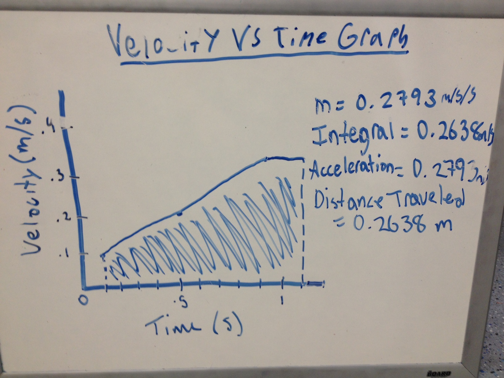
At the outset of our task to build this model, the students did a simple activity where they graphed the angle of rotation of a wooden disk with the distance the disk rolled across a flat surface. When they graphed the angle through which the wheel turned to the distance the wheel rolled, they found that the radius of the wheel was the slope. This meant that the linear displacement of a rolling object could be related to the angular displacement and likewise, the rate of these displacements were related through the radius.

Turning Effect

Once we had established some understanding around angular displacement, we started this model by investigating the conditions under which a rigid body’s rotational motion changed and when it didn’t change. I want to thank Sam for his post on how to begin investigating a turning effect.The students essentially followed this line of questioning and observing to establish a set of rules for defining when a rigid body’s rotational motion state will change. This lead the students to first make the claim that a change in “turning” was due to an unbalanced force acting on the wheel (especially those forces acting at a right angle to the radius!). The “turning” didn’t seem to change much when the forces acting on the wheel were balanced.

Uh, The Forces Aren’t Balanced, But The Thing Isn’t Turning?

The next class, I set up a simply “see-saw” with a meter stick and two different masses placed at different locations so that the meter stick didn’t rotate. I then asked the students if the forces were balanced. They immediately replied – “no”. So what gives? Students immediately saw that the Force Particle Models were not sufficient in dealing with rigid body motion, and many immediately suggested that the distance from the center of rotation also affected the “turning effect”. This discovery lead to a discussion about particles.

Extended Rigid Bodies vs. Particles

All the models that we had built in the past assumed that an object could be simplified by accepting that all the mass of the object could be identified as being located at a single point, namely the center of mass, because each particle of mass located in an object was experiencing the same linear motion state. The problem with a rotating object is that most points within a rotating object are actually traveling with different linear velocities (and accelerations). We needed a new way to define the basic constituent of this model. I suggested that we stick to as simple a definition as possible – a rigid extended body. This could be identified by a straight line (or lines) passing through a rotation point. The length represented an “un-bendable, un-squishable” collection of particles extending from the center of rotation outward to any edge of the extended body.

The Moment For The Moment Arm

This set us up for the next investigation. I asked the students to create an investigation where they had to prove that there was a connection between the force and the location that force was being applied and the turning effect. Students at first struggled to create an investigation that demonstrated a functional (input=output) relationship. Many students found evidence that supported their hypothesis, but I had to explain that these were not conclusive because it was limited to a single data point. This lead to a rich whiteboard session where students worked through the process of designing an experiment that went beyond describing a single situation. I’d like to return to this at a later point regarding scientific reasoning, but that is going to have to wait. Students eventually graphed the output force required when the input distance from the center of rotation was changed – in order for the system’s rotational motion state to be unchanged. This also quickly lead to the question of direction. It seemed that the force direction in relation to the radius of rotation seemed to affect the rotational state of the meter stick. At this point I introduced the concept of Torque and we discussed the vector cross product. I think for future classes, I’d like to introduce the cross product a bit differently. Using the line of action (as is done sometimes by engineers) seems to be a more useful method – at least visually – in explaining why the angle of the force is also part of what defines the torque value.

Deploying The Model (Part 1):

To test the model (thus far), the students were given a meter stick with a small weight attached to one end. The students then had to predict the point at which the meter stick could be moved off the edge of a table before rotating, and thus fall off. This allows the students to see the importance of identifying the gravitational force on the stick as affecting the turning effect around a point of rotation – which in this case was clearly not the center of mass of the stick. After some challenges, the students were mostly able to predict the point at which their meter sticks could be pushed before falling off the table. Next time, I’d like to reinforce this by also doing an experiment where two force meters support a meter stick with weights placed at different locations along the meter stick and have the students predict the forces read by both force meters. It was now time to look at situations where the torques were unbalanced. On to the second part of the model.