Testing Motors For The Solar Dragster Race

Torque/Speed Curves

In this post I’m going to describe our attempt to measure the power curve for the DC motors used in the Solar Dragster race this year. I’m going to be honest, our efforts weren’t really that successful, but I can at least say that I learned some things that might help for next year, and I think the students were able to do some authentic device testing – a part of being an engineer.

Last year I was a bit concerned that the DC motors that we were using in the Solar Dragster Race were not actually outputting the same power. I wanted to devise a way to measure the motor power, and then have each team do their own analysis. I wanted the students to do this without understanding the electrical power parameters involved because we were at this point only looking at motors as being a black box that gets energy from a source and transfers that energy into a rotational device – i.e. an axle, then to a gear, then to another axle, and finally to a wheel. I looked into getting a torque sensor, but quickly found out that these cost a fortune!

I came across this interesting website from MIT, which was a nice resource for the theory about DC motor performance. The site does a nice job in explaining torque/speed curves, and how the graph of torque vs angular speed is essentially linear for DC motors. That meant that all the students really needed to do was to measure stall torque and the no load speed of their motors and then we would have the torque/speed curve. The website identifies a device that they custom built for testing motors, and it looks interesting, but I didn’t have time to reverse engineer what they had built and unfortunately the images and videos aren’t clear enough to easily understand how the device works – something perhaps for summer tinkering…

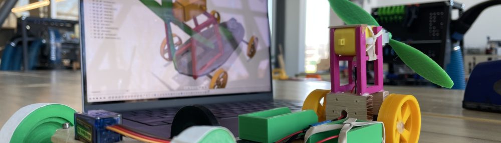
One of the issues with the little DC motors that you buy is that the arbor is really small, and it has no index, so its really hard to attach anything. Generally, you have to go with a friction fitting, and I was worried that doing a stall torque test was going to be difficult. Mr. Holt and I designed and printed out a little lever arm to attach to the motors. This little arm could then be attached to a force meter to measure the stall torque and then also used to help measure the rotational velocity using a Photogate. The final “test-bench” looked like this:

Torque-speed test bench

The motors were clamped to a lab stand that was then placed so that the little lever arm would rotate and block the Photogate laser as it spun. This is how the students measured the no load speeds. Then they attached a string to the little hole in the arm, and then attached this to a force meter to get the stall torque. All the motors were tested with essentially the same power source – two AA batteries.

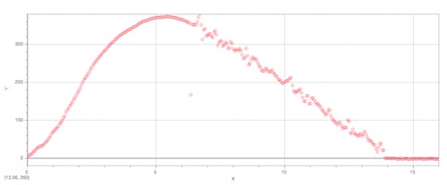
I then had the students share their data using a Google Spreadsheet and I compiled the data – here it is on Plotly:

dc_motor_tests

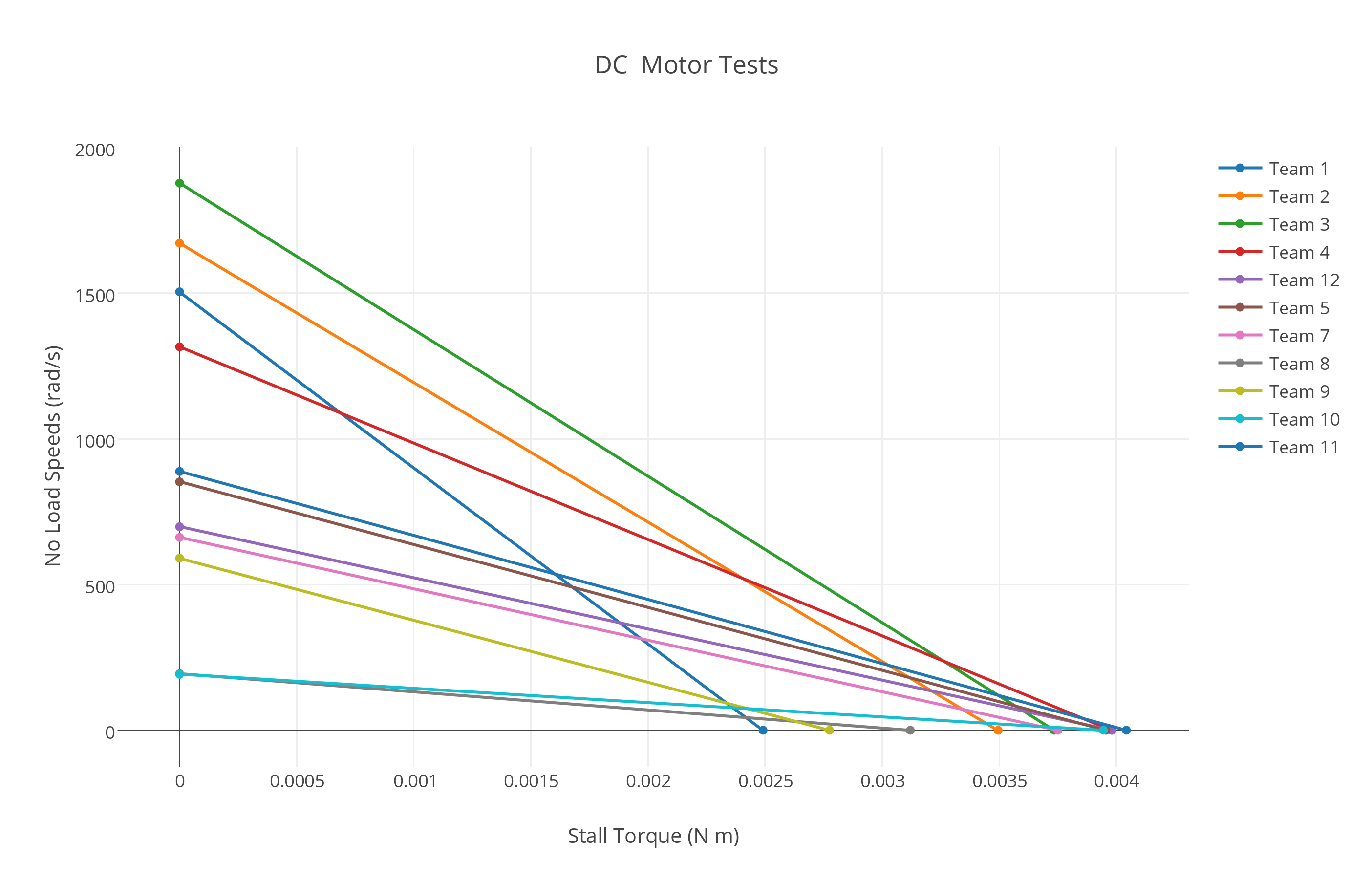
There is obviously some variability in the motor performance, but its hard to tell if any of the motors give a distinctive advantage over the others because I suspect that the data is not that reliable unfortunately. I do suspect that the angular speed data might be inaccurate due to the fact that we were getting some very differing results from the Photogate. Although we made the sampling rate as rapid as possible, I still am not confident that the Photogate was able to read the blocking of the laser accurately – the motors spin VERY fast (upwards of 5000 RPM’s when not loaded). I’m also not sure if the data then could then be used in any instructive way to help students make design decisions about their dragsters.

Although this may seem like a failure, it did allow the students to identify at least two motors that we knew were malfunctioning, so we were able to swap those out before the competition.

For Next Year

I think at this point I would want to make some changes to this activity. Although it was somewhat helpful in giving the students a direct interaction with data associated with the performance of a DC motor, and how that performance is calculated at the product of the torque and angular velocity, I’m not sure that the activity supplied data that was good enough to then use as an input factor in the competition. For example, I didn’t feel confident about allowing students to use the calculated maximum input power as a scaling factor for their dragster race time.

Perhaps next year, we can find the funds to purchase a high precision, digital torque meter, or find the time and money to build our own “analog” torque/speed meter like the one that MIT designed. All in all, I’d say this activity was partially successful.

Building The Net Torque Model – Part 3

Appending The Conservative Models

After investigating the causal relationship between torque and angular acceleration, I introduced the possibility to the class that perhaps we also needed to revisit the Energy Transfer Model and the Momentum Transfer Model. The students agreed that an object that is rotating must have energy. This was pretty easy to demonstrate.

I set up a situation in the class where two of the variable inertia disks that we created on the 3D printers were placed at the top of an inclined ramp. The internal marbles were placed at two different configurations inside the disks and then the students predicted which disk would reach the end of the ramp first. I was pleased to find out that the class appeared to agree that the disk with the marbles located closer to the radius would be the winner. I really think that our investigation with the variable inertia disks solidified the students’ conceptual understanding of rotational inertia and the importance of mass distribution.

I have not yet found a good experiment where students could discover the rotational kinetic energy relationship, so I decided to take them through a derivation based on linear kinetic energy. I then asked the students to do some whiteboard work. I asked them to demonstrate that the disks would indeed reach the end of the ramp at different times. Although this wasn’t strictly a constructivist approach, it was good practice in doing some fairly difficult algebra without numerical values – something the students traditionally are not very good at.

We then moved onto momentum. Again, I started by reviewing the Momentum Transfer Model for a particle. At this point the pattern had been fairly well established. The relationship between angular and linear quantities seemed to have taken hold because the students were quick to propose a mathematical definition for angular momentum. Our next goal was to figure out whether this was a conserved quantity.

Mr Holt and I had created a set of metal disks that could be attached to the rotary sensors. I decided to create our own, rather than (sorry Vernier) buy them as I thought that the commercial kit was over priced. It wasn’t too hard to create the disks, especially when you have access to a CNC plasma cutter!

image1

The students attached one disk to the rotary motion sensor and then got that disk spinning. They then took a second disk that had small magnets attached to it, and dropped this disk onto the spinning disk. The students compared the angular velocity before and after the disks were combined and then calculated the angular momentum of the system before and after. The data we got was quite good with the class getting in the range of only about a 5% to 6% difference.

Wrapping it Up (or Un-Rolling It Down)

As a final deployment, I decided to try the deployment activity that Frank Nochese did with his students. It seemed like a good (and fun) way to wrap up our model (or as I have already argued – models).

Before doing the deployment activity, I reviewed all the model specifics with the students. My point here was to impress on them that what we had not really built a new model, but rather had extended many of the prior particle models to include rigid extended bodies. This generally only required that we consider the moment arm in all the particle models. I think this really helped a number of students see the connection between models that they felt they understood and all this rotational stuff that seemed a bit confusing.

I then set them up with the deployment activity, but I asked them to specifically solve the problem using both energy and net torque. There was some success, but I realized that the task was a bit much for the class. Once again, it is clear that I need to give them more practice with these problems that require multiple steps and that involve algebraic manipulation of symbols without numbers. Plenty of time to practice that!

Building The Net Force Particle Model (Part 1)

From “The How” to “The Why”:

One of the three projects that the students will complete this year is a custom designed and fabricated rocket. One of the requirements of this project is for the rockets to carry a small solid state altimeter that collects vertical position data. This year I decided to give the students some data collected by last year’s students. Here is what the data looks like from one typical altimeter reading:

Rocketdata2013

As an introduction to this next model, I presented them with the data and asked them to use both the Constant Velocity Particle Model and the Constant Acceleration Particle Model to describe the motion of the rocket based on the data. Students responded to several questions that I created and they posted their answers through the Learning Management System we use.

A Simple Definition, A Simple Representation

The student investigation teams were then asked to draw velocity vs time graphs on their whiteboards. I was impressed to see that most teams were able to interpret the position data and create a velocity graph that agreed with the data. There was some debate about the graphs, but the students worked through these differences and came to consensus around what the graph would most likely look like. At this point I was thinking about using LoggerPro’s ability to graph the derivative of a data set, but decided that I would leave that for a later date, though next year I might do it earlier.

I then introduced a very basic definition of a force:

“A Force is A Push or A Pull”

And then I proposed that we could represent the force with an arrow, just as we had done with velocity and acceleration. I then asked them to divide the rocket data into four sections based on the answers to the questions we had discussed. The students then drew a representation of the rocket in each stage and the forces acting on the rocket. The stages the students identified were 4) on the ground, 3) descending by parachute, 2) going up without fuel, and 1) going up with fuel. I asked them to draw the diagrams by starting at the end. Here is a typical example of the force diagrams the students drew:

photo 2

The labeling is a standard that is outlined in the Modeling methodology – it reads (type, feeler, dealer).

Constant Velocity Motion and Net Force

We started the class discussion by looking at the forces acting on the rocket when the rocket was on the ground. Students agreed unanimously that there were two forces acting on the rocket – one down, one up – the gravitational force and then the force from the ground. Great. Then on to the descent phase. Certainly less unanimity here. The students again agreed on the number of forces – two – one up from air resistance, one down from gravity. The students quickly got into several back-and-forth arguments about the length of the force vectors. The class was split. Were the forces equal? Or, was gravity “winning”? The big stumbling block was around the question, “if gravity was equal to the air resistance force, then why was the rocket still falling”? A classic example of Aristotelian thinking. I encouraged them to ask the question – “if gravity was winning, why wasn’t the rocket speeding up?” One student proposed that maybe the force of gravity was just ever so slightly larger. Some students pounced in this. They argued that the forces weren’t equal at first, but as the rocket (with parachute) descended, the air resistance force strengthened and eventually became as strong as the gravitational force. the reason the rocket didn’t slow down was because it was already moving when the forces became equal. Awesome. Then a student gave an excellent description of a thought experiment where a box was traveling through space in one direction and convinced the students that the box would not slow down if you pushed equally on both sides of the box. Students reached consensus – the rocket moved at a constant velocity because the forces were equal.

The “Residue” Misconception

We then progressed to the next stage. Things got really interesting. Without exception, ALL the student groups identified an arrow pointing upward, even though they all agreed that the fuel had run out. The question that I think cuts through this the quickest is to ask “who is pushing on the rocket upward?” Most students get that funny look on their faces as their brains begin to realize that they just ran into a logical conundrum. Some students start to respond – “the rocket pushes the rocket.” OK, how? What kind of force is it? A contact force? How does it push or pull itself? The students at this point began to question each other and the room erupted in arguments. Being a bit of a control freak, I’ve had to learn to allow space and time for these chaotic moments, but also realize the importance of catching the class before it descends into something less productive.

At this point, one group erased the upward force. I asked them why they had done this. They responded that they didn’t think a force was needed for the rocket to continue upward, and that gravity and air resistance were slowing the rocket down. This seemed impossible to some of the students. They asked – “but something is left over after the fuel runs out, isn’t there?” The class began to divide up into those that now believed the rocket no longer had any upward force acting on it and those that believed there was some kind of “left-over” force, what I call a “residue”. So, once again, I asked them to identify the dealer of the residue force. The answer is generally – “the fuel”. Ah, but hasn’t the fuel run out? Yes, but the rocket has gained something from the fuel and now that is what is pushing it upward.

This is not such a wild idea, and in fact is not that far from the idea of Kinetic Energy. The students that were in the “no upward force” camp started to explain to the other students in the class that the fuel had “given” the rocket its upward velocity, but now that the fuel was gone, the rocket was now slowing down. We discussed the idea that anything that was slowing down must be experiencing a force pushing in the opposite direction of its velocity. We returned to the thought experiment with the box floating through space. The students debated about whether this box would slow down if the force that had gotten the box moving in the first place disappeared. The students agreed that if there were no forces acting on it to slow it, then it was reasonable to say that it would never slow down. Students then agreed the rocket was no different. It didn’t need a force to continue moving at a constant velocity, but that if it was instead accelerating (in this case in the negative direction) then it would need a force, which was provided by gravity and the air resistance force.  The students began to coalesce around the idea that if a force was a push or a pull, then the rocket that had run out of fuel was not getting pushed any longer, and that although it was moving upward it was indeed accelerating downward.

Making Some Observations

During the next class, I had the students set up a motion detector on one side of a Vernier dynamics track and use a force meter to pull on a low friction cart. They were to also record the velocity of the cart while the students pulled twice in quick succession on a string connected to the cart and force meter.

IMG_0686

The students then shared their graphs with the rest of the class:

IMG_0687

This experiment is meant to re-enforce some of the arguments made during the previous class. The students quickly see that the velocity is measured to change when the force is applied and that the velocity is “constantish” when no force is applied. The students were ready to tackle how the force and acceleration were quantitatively related, but that’s for another post…